2 Optimization Problems
The goal of an optimization problem is to minimize or maximize an objective function subject to constraints. A minimization problem has the form:
\begin{alignedat}{2} \text{minimize} \quad & f(\mathbf{x}) \\ \text{subject to} \quad & g_i(\mathbf{x}) \leq 0, &\qquad& i = 1, \ldots, m \\ & h_j(\mathbf{x}) = 0, && j = 1, \ldots, p \end{alignedat}
Here, \mathbf{x} \in \mathbb{R}^n is the vector of decision variables, and f:\mathbb{R}^n \to \mathbb{R} is the objective function. The aim is to find \mathbf{x} that minimize f(\mathbf{x}) while satisfying all constraints.
The constraints g_i(\mathbf{x}) \leq 0 are called inequality constraints, and h_j(\mathbf{x}) = 0 are equality constraints. The terms “minimize” and “maximize” are often abbreviated as “min” and “max,” respectively, and “subject to” is abbreviated as “s.t.”
A solution is feasible if it satisfies all constraints. The set of all feasible solutions is called the feasible region. For a minimization problem, a feasible solution \mathbf{x}^* is optimal if it achieves the smallest objective value among all feasible solutions.
Example 2.1 (An Example of an Optimization Problem) Consider the following optimization problem:
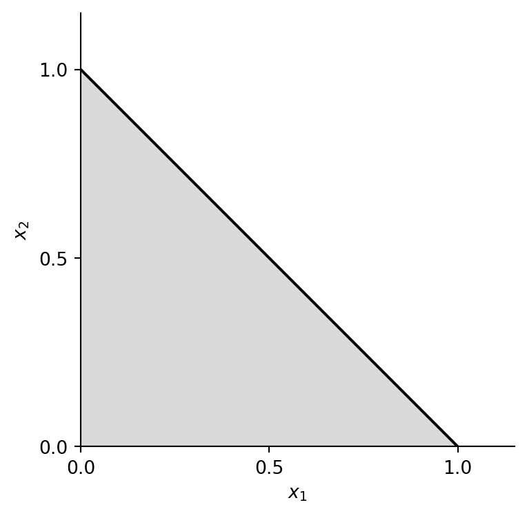
\begin{aligned} \min \quad & x_1^2 + x_2^2 \\ \text{s.t.} \quad & x_1 + x_2 \leq 1 \\ & x_1 \geq 0 \\ & x_2 \geq 0 \end{aligned}
Figure 2.1 shows the feasible region of this optimization problem. The optimal solution is at the point (0, 0).
2.1 Linear Programming
A linear programming (LP) problem has a linear objective function, linear constraints, and continuous decision variables. It can be written as:
\begin{aligned} \min \quad & \mathbf{c}^{\top} \mathbf{x} \\ \text{s.t.} \quad & \mathbf{A} \mathbf{x} \leq \mathbf{b} \\ & \mathbf{x} \geq 0 \end{aligned}
Example 2.2 (The Diet Problem) Consider a diet problem where the objective is to minimize the cost of food while meeting the nutritional requirements. Suppose there are n types of food and m types of nutrients. Let c_j be the cost per unit of food j, a_{ij} be the amount of nutrient i per unit of food j, and b_i be the minimum required amount of nutrient i. Table 2.1 shows the amounts a_{ij}.
| Food 1 | Food 2 | … | Food n | |
|---|---|---|---|---|
| Nutrient 1 | a_{11} | a_{12} | … | a_{1n} |
| Nutrient 2 | a_{21} | a_{22} | … | a_{2n} |
| … | … | … | … | … |
| Nutrient m | a_{m1} | a_{m2} | … | a_{mn} |
Let x_j be the amount of food j to consume. The diet problem can be formulated as:
\begin{alignedat}{2} \min \quad & \sum_{j=1}^{n} c_j x_j \\ \text{s.t.} \quad & \sum_{j=1}^{n} a_{ij} x_j \geq b_i, &\qquad& i = 1, \ldots, m \\ & x_j \geq 0, && j = 1, \ldots, n \end{alignedat} \tag{2.1}
The objective is the total food cost. The constraints ensure that each nutrient requirement is met and that food quantities are nonnegative.
Let \mathbf{A} be the m \times n matrix with entries a_{ij}, \mathbf{b} be the vector of minimum required nutrient amounts, and \mathbf{c} be the vector of unit food costs. Let \mathbf{x} be the vector of decision variables. Then, we can write the diet problem as:
\begin{aligned} \min \quad & \mathbf{c}^{\top} \mathbf{x} \\ \text{s.t.} \quad & \mathbf{A} \mathbf{x} \geq \mathbf{b} \\ & \mathbf{x} \geq 0 \end{aligned}
2.2 Mixed-Integer Programming
In a mixed-integer programming (MIP) problem, some decision variables are required to be integers. With a linear objective and linear constraints, the model takes the form:
\begin{aligned} \min \quad & \mathbf{c}^{\top} \mathbf{x} + \mathbf{d}^{\top} \mathbf{y} \\ \text{s.t.} \quad & \mathbf{A} \mathbf{x} + \mathbf{B} \mathbf{y} \leq \mathbf{b} \\ & \mathbf{x}, \mathbf{y} \geq 0 \\ & \mathbf{x} \in \mathbb{Z}^{n} \end{aligned}
Here, \mathbf{x} contains the integer variables and \mathbf{y} the continuous variables. If all decision variables must be integers, the problem is called an integer programming (IP) problem.
2.2.1 The 0-1 Knapsack Problem
The 0-1 knapsack problem is a classic example of an integer programming problem. In this problem, we have n items, each with a weight w_j and a value c_j. Given a knapsack with a maximum weight capacity K, we want to select items to maximize the total value without exceeding the weight capacity. Define a binary decision variable x_j for each item j, where x_j = 1 if item j is selected and x_j = 0 otherwise.
The 0-1 knapsack problem can be formulated as:
\begin{alignedat}{2} \max \quad & \sum_{j=1}^{n} c_j x_j \\ \text{s.t.} \quad & \sum_{j=1}^{n} w_j x_j \leq K \\ & x_j \in \{0, 1\}, &\qquad& j = 1, \ldots, n \end{alignedat}
2.2.2 Facility Location Problem
Sets
- I: Set of clients
- J: Set of potential facility locations
Parameters
- c_j: Fixed cost of opening facility j \in J
- d_{ij}: Cost of serving client i \in I from facility j \in J
Decision Variables
- y_j: 1 if facility j is opened, and y_j = 0 otherwise.
- x_{ij}: 1 if client i is served by facility j, and 0 otherwise.
The uncapacitated facility location problem (UFLP) can be formulated as follows:
\begin{alignedat}{2} \min \quad & \sum_{j \in J} c_j y_j + \sum_{i \in I} \sum_{j \in J} d_{ij} x_{ij} \\ \text{s.t.} \quad & \sum_{j \in J} x_{ij} = 1, &\qquad& i \in I \\ & x_{ij} \leq y_j, && i \in I, j \in J \\ & x_{ij} \in \{0, 1\}, && i \in I, j \in J \\ & y_j \in \{0, 1\}, && j \in J \end{alignedat}
Here, \sum_{j \in J} x_{ij} = 1 ensures that each client is served by exactly one facility. The forcing constraint x_{ij} \leq y_j ensures that a client can only be served by an open facility (Why?).
2.2.3 Wagner-Whitin Model
Sets
- \mathcal{T}: The set of time periods, \mathcal{T} = \{1, 2, \ldots, T\}
Parameters
- K: Ordering cost per order
- h: Holding cost per unit
- d_t: Demand in period t
- M: A large positive number
Decision Variables
- q_t: Order quantity in period t
- x_t: Inventory level at the end of period t
- y_t: Binary variable indicating whether an order is placed in period t. y_t = 1 if an order is placed, and y_t = 0 otherwise.
Define x_0 = 0 as the initial inventory level. The Wagner-Whitin model can be formulated as follows:
\begin{alignedat}{2} \min \quad & \sum_{t=1}^{T} (K y_t + h x_t) \\ \text{s.t.} \quad & x_t = x_{t-1} + q_t - d_t &\qquad& t \in \mathcal{T} \\ & q_t \geq 0 && t \in \mathcal{T} \\ & q_t \leq M y_t && t \in \mathcal{T} \\ & x_t \geq 0 && t \in \mathcal{T} \\ & y_t \in \{0, 1\} && t \in \mathcal{T} \end{alignedat}
Here, the constraint q_t \leq M y_t is a Big-M constraint that ensures that if y_t = 0, then q_t = 0 (i.e., no order is placed). If y_t = 1, then q_t can take any value up to M.
2.3 Problem and Instance
It is important to distinguish between a problem and an instance of a problem. Informally, an instance has specific input data for the parameters of a problem so that the problem can be solved for that particular set of data; while a problem is a collection of instances.
Definition 2.1 An instance of an optimization problem consists of a feasible set \mathcal{X} and a cost function f: \mathcal{X} \to \mathbb{R}. The objective is to find a \mathbf{x} \in \mathcal{X} that f(\mathbf{x}) \leq f(\mathbf{y}), \quad \forall \mathbf{y} \in \mathcal{X}.
An optimization problem is a collection of instances.
2.4 Neighborhoods
Definition 2.2 Given an optimization problem with a feasible region \mathcal{X}, a neighborhood is a mapping
N: \mathcal{X} \to 2^{\mathcal{X}}.
Example 2.3 For a linear programming problem, a common neighborhood definition is:
N(\mathbf{x}) = \{\mathbf{y} \in \mathcal{X} : \|\mathbf{y} - \mathbf{x}\| \leq \epsilon\}
where \epsilon > 0 is a small constant. The neighborhood of \mathbf{x} consists of all feasible solutions \mathbf{y} that are within Euclidean distance \epsilon of \mathbf{x}.
2.5 Local and Global Optima
Definition 2.3 Given an optimization problem with a neighborhood N, a feasible solution \mathbf{x} \in \mathcal{X} is a local optimum with respect to N if
f(\mathbf{x}) \leq f(\mathbf{y}), \quad \forall \mathbf{y} \in N(\mathbf{x}).
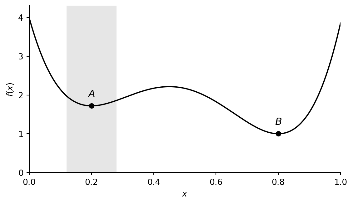
Example 2.4 Consider the optimization problem given in Figure 2.2. Define the feasible region \mathcal{X} = [0, 1], and the neighborhood N(x) = \{y \in \mathcal{X} : |y - x| \leq \epsilon\}. Then, the points A and B are both local optima with a small enough \epsilon. Furthermore, B is the global optimum.
2.6 Single-objective vs Multi-objective Optimization
So far, we have considered problems with a single objective function. In many real-world applications, we have multiple objectives that we want to optimize simultaneously. This is called multi-objective optimization. The general form of a multi-objective optimization problem is:
\begin{alignedat}{2} \min \quad & (f_1(\mathbf{x}), f_2(\mathbf{x}), \ldots, f_k(\mathbf{x})) \\ \text{s.t.} \quad & g_i(\mathbf{x}) \leq 0, &\qquad& i = 1, \ldots, m \\ & h_j(\mathbf{x}) = 0, && j = 1, \ldots, p \end{alignedat}
where f_1, f_2, \ldots, f_k are the objective functions. When k = 2, this is called bi-objective optimization.
The objectives may conflict, that is, improving one can worsen another. We therefore often need to consider trade-offs between objectives.
2.7 Applications
- Supply chain management
- Inventory management
- Production planning
- Transportation
- Scheduling
- Deep learning
- Engineering design
- Healthcare
- Finance
- …
2.8 Optimization in Artificial Intelligence
Nowadays, one of the most important applications of optimization is in artificial intelligence (AI). Many AI problems can be formulated as optimization problems.
In supervised learning, we often want to minimize a loss function to find the best model parameters. Optimization algorithms (or optimizers) such as stochastic gradient descent (SGD) and Adam are widely used in deep learning frameworks like PyTorch and TensorFlow.
In reinforcement learning, we want to maximize the expected reward by finding the optimal policy. The study of reinforcement learning is closely related to dynamic programming.
2.9 Optimization Methods
- Exact methods
- Heuristic methods
2.10 How to Solve Optimization Problems
There are several methods for solving optimization problems:
Optimization problems can be solved in several ways:
Manual methods: Small, simple problems can be solved by hand using graphical methods or algorithms such as the simplex method.
Optimization solvers: Commercial and open-source software, such as Gurobi, CPLEX, COPT, and tools from COIN-OR, can solve many optimization problems. These tools often provide APIs for languages such as Python, C, and Java. Their performance depends on the size and structure of the problem. See this list of optimization software for more details.
Problem-specific algorithms: Algorithms that exploit the structure of the problem can improve efficiency, especially when general-purpose solvers struggle. Depending on the approach, these algorithms may provide exact or satisfactory solutions. The development of problem-specific algorithms is an active area of research in operations research and optimization.
There are also libraries that focus on optimization in specific domains, as listed in Table 2.2.
| Domain | Libraries |
|---|---|
| Hyperparameter optimization | Optuna |
| Vehicle routing | pyVRP |
| Portfolio optimization | PyPortfolioOpt |
| Inventory management | PyInventory |
| Job shop scheduling | PyJobShop |
2.11 Benchmark Problems
2.11.1 Operations Research Problems
Table 2.3 lists benchmark instances for some well-known operations research problems.
| Problem | Benchmark |
|---|---|
| Traveling Salesman Problem (TSP) | TSPLIB |
| Capacitated Vehicle Routing Problem (CVRP) | CVRPLIB |
| Job Shop Scheduling Problem (JSSP) | Taillard’s Benchmark, Demirkol’s Benchmark |
OR Library collects benchmark instances for various OR problems. Job Shop Scheduling is actively maintained and provides the lower and upper bounds for the well-known benchmark problems. SimOpt is a repository of simulation optimization problems.
2.11.2 Black-box Optimization Problems
Congress on Evolutionary Computation (CEC) is a conference that hosts competitions on black-box optimization problems. The CEC suites are widely used as benchmarks for optimization algorithms.
pymoo provides a collection of test problems for single-objective, multi-objective optimization.
BBOB is a benchmark suite for black-box optimization problems, which is part of the COCO platform. The COCO platform has been used in the GECCO conference.