30  Simulated Annealing

While the local search algorithm guarantees the local optimality of the solution, the solution may not be globally optimal. Simulated annealing is designed to improve the local search by escaping local optima by occasionally accepting worse solutions.

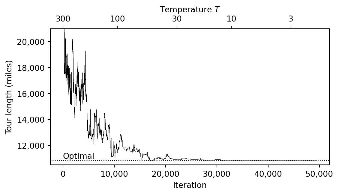
Figure 30.1 illustrates this idea. Local search moves only to better neighbors, so it stops at the local optimum at the bottom of the left valley. To reach the global optimum, the search must first move to worse solutions to get out of this valley.

Code
import matplotlib.pyplot as plt
import numpy as np

# Solutions 0, 1, ..., 24 on a line. The neighbors of solution k are k - 1 and k + 1.
# The objective function has a shallow valley around 6 and a deep valley around 18.
k = np.arange(25)
f = (
    9
    + 0.004 * (k - 12) ** 2
    - 4 * np.exp(-(((k - 6) / 2.6) ** 2))
    - 8 * np.exp(-(((k - 18) / 3) ** 2))
)
start, local_opt, global_opt = 1, 6, 18

fig, ax = plt.subplots(figsize=(6, 3.5))
ax.plot(k, f, color="black", linewidth=0.8, zorder=1)
ax.scatter(k, f, s=28, color="white", edgecolor="black", linewidth=0.8, zorder=2)
ax.scatter(start, f[start], s=28, color="black", zorder=3)

# Draw the moves slightly above the solutions, with an arrowhead at the end
for path, linestyle in [
    (np.arange(start, local_opt + 1), "-"),  # local search: downhill only
    (np.arange(local_opt, global_opt + 1), "--"),  # simulated annealing
]:
    y = f[path] + 0.5
    ax.plot(path, y, color="black", linestyle=linestyle, linewidth=1.5)
    ax.annotate(
        "",
        xy=(path[-1], y[-1]),
        xytext=(0.1 * path[-2] + 0.9 * path[-1], 0.1 * y[-2] + 0.9 * y[-1]),
        arrowprops=dict(
            arrowstyle="-|>", color="black", mutation_scale=12, shrinkA=0, shrinkB=0
        ),
    )

for x, label, offset in [
    (start, r"$\mathbf{x}^{(0)}$", (-4, -16)),
    (local_opt, "Local optimum", (0, -18)),
    (global_opt, "Global optimum", (0, -18)),
]:
    ax.annotate(
        label, xy=(x, f[x]), xytext=offset, textcoords="offset points", ha="center"
    )
ax.text(2.6, f[3] + 1.3, "Local search")
ax.text(11.4, f[11] + 1.0, "Simulated annealing:\noccasionally accepts\nworse solutions")

ax.set(
    xlabel=r"Solution $\mathbf{x}$",
    ylabel=r"$f(\mathbf{x})$",
    xticks=[],
    yticks=[],
    xlim=(-0.8, 24.8),
    ylim=(f.min() - 2, f.max() + 4.2),
)
ax.spines[["top", "right"]].set_visible(False)
fig.tight_layout()
plt.show()
Line chart of the objective value f(x) of 25 solutions, drawn as open circles connected by a thin line, with no axis ticks. The line has two valleys separated by a ridge: a shallow valley on the left, whose lowest circle is labeled Local optimum, and a deeper valley on the right, whose lowest circle is labeled Global optimum. A thick solid arrow labeled Local search starts at the filled circle x(0), the second circle from the left, and goes down the left valley to the local optimum. A dashed arrow starts at the local optimum, climbs over the ridge, and goes down to the global optimum. It is labeled Simulated annealing: occasionally accepts worse solutions.
Figure 30.1: A one-dimensional example. Each circle is a solution, and the line connects neighboring solutions. Local search from \mathbf{x}^{(0)} stops at a local optimum. The dashed path shows how simulated annealing can leave it by moving to worse solutions.

Simulated annealing was proposed by Kirkpatrick et al. (1983), and it was used to solve VLSI layout problems in the 1980s (Rutenbar 1989). This algorithm is related to the Metropolis algorithm (Metropolis et al. 1953).

Let \mathbf{x} be the current solution and \mathbf{y} \in N(\mathbf{x}) be a neighboring solution chosen at random. Solution \mathbf{y} can be either a better solution or a worse solution than \mathbf{x}. Let \Delta f = f(\mathbf{y}) - f(\mathbf{x}) be the change in the objective value. If \Delta f < 0, the algorithm always moves to the better solution \mathbf{y}. Otherwise, it moves to \mathbf{y} with a probability

e^{-\Delta f / T}.

Here, T > 0 is a parameter called the temperature. To understand the intuition of this probability, we first consider a fixed temperature T. The larger the difference \Delta f, the smaller the probability of moving to the worse solution \mathbf{y}.

The temperature T controls the probability of moving to a worse solution. With a small temperature T, the probability of moving to a worse solution is small, and the algorithm behaves like a local search. With a large temperature T, the probability of moving to a worse solution is large, and the algorithm explores the solution space more widely.

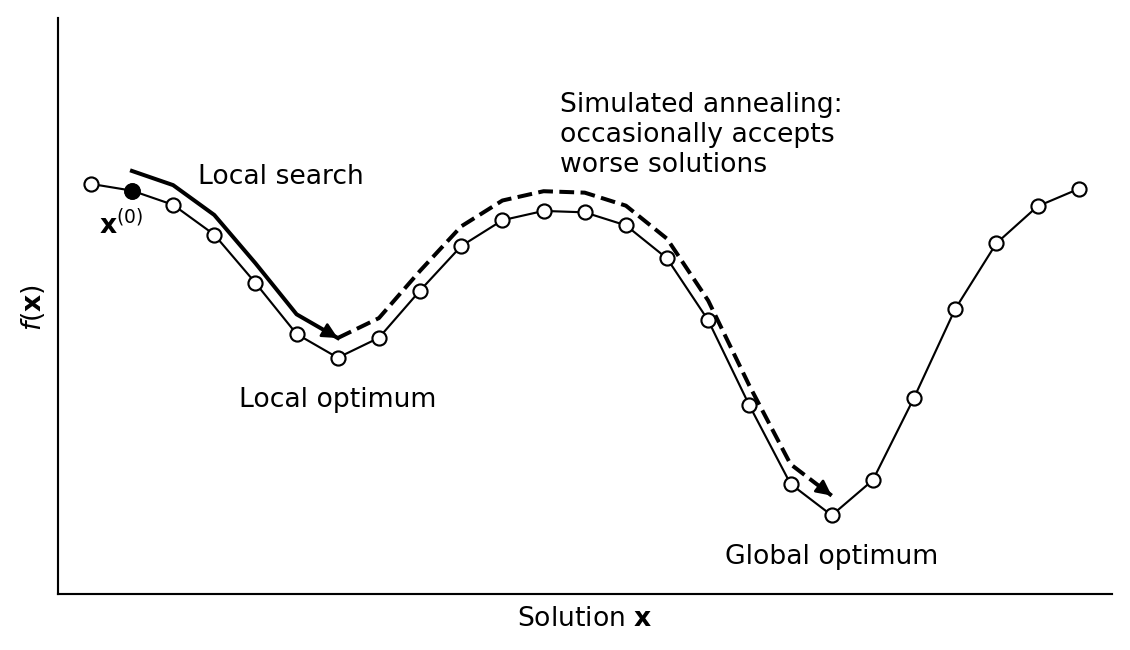
Figure 30.2 plots the probability e^{-\Delta f / T} against \Delta f for T = 0.5, 1, 2, and 5.

Code
import matplotlib.pyplot as plt
import numpy as np

delta = np.linspace(0, 5, 501)
temperatures = [0.5, 1, 2, 5]

fig, ax = plt.subplots(figsize=(6, 3.5))
for T in temperatures:
    ax.plot(delta, np.exp(-delta / T), color="black")
    # Label each curve at delta = 1, where the curves are well separated
    ax.annotate(
        f"$T = {T}$",
        xy=(1, np.exp(-1 / T)),
        xytext=(4, 4),
        textcoords="offset points",
    )
ax.set(
    xlabel=r"$\Delta f = f(\mathbf{y}) - f(\mathbf{x})$",
    ylabel=r"Probability of accepting $\mathbf{y}$",
    xlim=(0, 5),
    ylim=(0, 1.05),
)
ax.spines[["top", "right"]].set_visible(False)
fig.tight_layout()
plt.show()
Line chart of the probability of accepting a worse solution against the difference Δf = f(y) − f(x), from 0 to 5, with one black curve for each temperature T = 0.5, 1, 2, and 5. All four curves start at probability 1 when the difference is 0 and decrease toward 0 as the difference grows. A higher temperature gives a higher curve: at a difference of 1, the probabilities are 0.14, 0.37, 0.61, and 0.82. At a difference of 5, the curves for T = 0.5 and T = 1 are nearly 0, while the curve for T = 5 is still at 0.37.
Figure 30.2: Probability of accepting a worse solution \mathbf{y} for four values of the temperature T.

The probability depends on \Delta f and T only through the ratio \Delta f / T. Thus, T has the same unit as f, and whether T is small or large depends on the typical size of \Delta f. For example, in the TSP of Section 30.2, the tour length is measured in miles, and a 2-opt exchange typically changes it by hundreds of miles, so T = 5 is a small temperature.

Overall, once \mathbf{y} has been chosen, the probability of accepting \mathbf{y}, that is, of moving from \mathbf{x} to \mathbf{y}, is given by the following formula:

p_{\mathbf{x} \mathbf{y}} = \begin{cases} 1 & \text{if } \Delta f < 0 \\ e^{-\Delta f / T} & \text{otherwise} \end{cases}

This probability is called the acceptance probability, and this rule is known as the Metropolis criterion (Metropolis et al. 1953).

In practice, the temperature T is gradually decreased during the search process, so that the algorithm explores the solution space widely at the beginning and gradually focuses on local search as the temperature decreases. The method of controlling the temperature T is called the annealing schedule.

The simulated annealing algorithm is summarized in Algorithm 1.

\begin{algorithm} \caption{Simulated Annealing} \begin{algorithmic} \Require initial solution $\mathbf{x}^{(0)} \in \mathcal{X}$, neighborhood $N$, initial temperature $T$, annealing schedule \Ensure best solution found $\mathbf{x}_{\text{best}}$ \State $\mathbf{x} \gets \mathbf{x}^{(0)}$ \State $\mathbf{x}_{\text{best}} \gets \mathbf{x}^{(0)}$ \While{stopping criterion not met} \State choose $\mathbf{y} \in N(\mathbf{x})$ at random \State $\Delta f \gets f(\mathbf{y}) - f(\mathbf{x})$ \If{$\Delta f < 0$ or $\text{random}(0, 1) < e^{-\Delta f / T}$} \State $\mathbf{x} \gets \mathbf{y}$ \EndIf \If{$f(\mathbf{x}) < f(\mathbf{x}_{\text{best}})$} \State $\mathbf{x}_{\text{best}} \gets \mathbf{x}$ \EndIf \State Update $T$ according to the annealing schedule \EndWhile \State \textbf{return} $\mathbf{x}_{\text{best}}$ \end{algorithmic} \end{algorithm}

30.1 Annealing Schedules

A common annealing schedule, known as the exponential (or geometric) annealing schedule, keeps the temperature T fixed for L iterations and then multiplies it by a factor \gamma \in (0, 1), i.e., T \gets \gamma T. A good choice is L = |N(\mathbf{x})|, the number of neighbors, and \gamma is typically between 0.8 and 0.99 (Delahaye et al. 2019).

30.2 Simulated Annealing for the TSP

We apply simulated annealing to the Car 54 instance of Chapter 29 with the 2-opt neighborhood. The following code defines the instance and the functions two_opt_move(), delta(), two_opt_moves(), tour_length(), first_improvement(), and local_search() in the same way as in Chapter 29.

Code
import numpy as np


def two_opt_move(tour, i, j):
    """Remove edges {tour[i], tour[i+1]} and {tour[j], tour[(j+1) % len(tour)]},
    and reconnect the tour by reversing tour[i+1], ..., tour[j]."""
    return tour[: i + 1] + tour[i + 1 : j + 1][::-1] + tour[j + 1 :]


def delta(tour, i, j, D):
    """Change in the tour length caused by two_opt_move(tour, i, j)."""
    n = len(tour)
    a, b = tour[i], tour[i + 1]
    c, d = tour[j], tour[(j + 1) % n]
    return D[a, c] + D[b, d] - D[a, b] - D[c, d]


def two_opt_moves(n):
    """All 2-opt moves (i, j) for a tour of n cities."""
    for i in range(n - 2):
        for j in range(i + 2, n):
            if i == 0 and j == n - 1:
                continue  # {tour[0], tour[1]} and {tour[n-1], tour[0]} are adjacent
            yield i, j


def tour_length(tour, D):
    """Length of the tour, including the edge back to the first city."""
    return sum(D[tour[k - 1], tour[k]] for k in range(len(tour)))


def first_improvement(tour, D):
    """Return the first improving move, or None if there is none."""
    for i, j in two_opt_moves(len(tour)):
        if delta(tour, i, j, D) < 0:
            return i, j
    return None


def local_search(tour, D, select):
    """2-opt local search. Return the local optimum and the tour lengths."""
    lengths = [tour_length(tour, D)]
    move = select(tour, D)
    while move is not None:  # while I(x) is not empty
        i, j = move
        tour = two_opt_move(tour, i, j)
        lengths.append(tour_length(tour, D))
        move = select(tour, D)
    return tour, lengths


# Name, latitude, and longitude of each city
cities = [
    ("Chicago, IL", 41.8500, -87.6500),
    ("Indianapolis, IN", 39.7667, -86.1500),
    ("Marion, OH", 40.5833, -83.1167),
    ("Erie, PA", 42.1167, -80.0833),
    ("Carlisle, PA", 40.2000, -77.1833),
    ("Wana, WV", 39.7000, -80.2833),
    ("Wilkesboro, NC", 36.1500, -81.1333),
    ("Chattanooga, TN", 35.0333, -85.3000),
    ("Barnwell, SC", 33.2333, -81.3500),
    ("Bainbridge, GA", 30.9000, -84.5667),
    ("Baton Rouge, LA", 30.4500, -91.1500),
    ("Little Rock, AR", 34.7333, -92.2833),
    ("Kansas City, MO", 39.0833, -94.5667),
    ("La Crosse, WI", 43.8000, -91.2333),
    ("Blunt, SD", 44.5000, -99.9833),
    ("Lincoln, NE", 40.8000, -96.6667),
    ("Wichita, KS", 37.6833, -97.3333),
    ("Amarillo, TX", 35.2167, -101.8167),
    ("Truth or Consequences, NM", 33.1167, -107.2500),
    ("Manuelito, NM", 35.4167, -108.9833),
    ("Colorado Springs, CO", 38.8333, -104.8167),
    ("Butte, MT", 46.0000, -112.5333),
    ("Lewiston, ID", 46.4167, -117.0167),
    ("Boise, ID", 43.6000, -116.2000),
    ("Twin Falls, ID", 42.5500, -114.4500),
    ("Salt Lake City, UT", 40.7500, -111.8833),
    ("Mexican Hat, UT", 37.1500, -109.8500),
    ("Marble Canyon, AZ", 36.8000, -111.6333),
    ("Reno, NV", 39.5167, -119.8000),
    ("Lone Pine, CA", 36.6000, -118.0500),
    ("Gustine, CA", 37.2500, -120.9833),
    ("Redding, CA", 40.5833, -122.3833),
    ("Portland, OR", 45.5167, -122.6667),
]

# Road distances in miles. Row i lists the distances from city i
# to cities 0, 1, ..., i - 1 (the lower triangle of D).
lower_triangle = [
    [184],
    [292, 195],
    [449, 310, 215],
    [670, 540, 380, 288],
    [516, 357, 232, 200, 211],
    [598, 514, 434, 566, 436, 381],
    [618, 434, 493, 787, 814, 642, 295],
    [881, 697, 719, 790, 632, 697, 224, 320],
    [909, 964, 955, 1020, 974, 952, 541, 341, 318],
    [978, 892, 1031, 1246, 1352, 1180, 843, 538, 747, 441],
    [654, 597, 803, 1018, 1154, 1104, 766, 461, 749, 634, 380],
    [504, 503, 722, 937, 1043, 806, 986, 722, 1042, 954, 784, 404],
    [276, 460, 568, 725, 946, 817, 874, 894, 1214, 1185, 1218, 660, 452],
    [780, 964, 1072, 1229, 1450, 1321, 1378, 1326, 1646, 1672, 1410, 1030, 626, 476],
    [529, 644, 789, 1004, 1184, 1001, 1214, 950, 1270, 1213, 1043, 632, 219, 436, 419],
    [805, 698, 917, 1132, 1238, 1055, 1113, 842, 1162, 1027, 779, 473, 195, 637, 634,
     256],
    [1181, 1007, 1226, 1441, 1547, 1364, 1375, 1080, 1134, 1138, 783, 611, 563, 1046,
     759, 624, 368],
    [1548, 1444, 1630, 1845, 1984, 1801, 1726, 1431, 1685, 1477, 1134, 1033, 906, 1389,
     1094, 967, 711, 404],
    [1547, 1454, 1668, 1883, 1994, 1811, 1879, 1584, 1776, 1632, 1267, 1053, 944, 1427,
     1196, 1005, 749, 442, 251],
    [1239, 1167, 1353, 1568, 1707, 1524, 1584, 1313, 1633, 1498, 1151, 979, 614, 988,
     600, 525, 471, 368, 512, 507],
    [1538, 1733, 1830, 2045, 2208, 2090, 2136, 2078, 2398, 2332, 2110, 1782, 1378, 1300,
     760, 1229, 1382, 1319, 1163, 930, 910],
    [1999, 2158, 2291, 2448, 2669, 2515, 2597, 2500, 2820, 2675, 2336, 2164, 1707, 1860,
     1375, 1582, 1658, 1545, 1389, 1156, 1237, 436],
    [1716, 1875, 2008, 2165, 2386, 2232, 2488, 2217, 2537, 2392, 2053, 1881, 1422, 1577,
     1106, 1244, 1375, 1262, 1106, 873, 954, 483, 283],
    [1580, 1738, 1872, 2029, 2250, 2095, 2352, 2081, 2401, 2256, 1917, 1745, 1286, 1473,
     988, 1147, 1239, 1126, 970, 737, 818, 379, 419, 136],
    [1425, 1569, 1717, 1874, 2109, 1926, 2115, 1844, 2164, 2019, 1680, 1508, 1118, 1335,
     862, 913, 1002, 889, 733, 500, 581, 430, 656, 373, 237],
    [1560, 1549, 1852, 2009, 2089, 1906, 2063, 1792, 2112, 1967, 1456, 1274, 1032, 1540,
     1068, 1007, 944, 665, 521, 282, 491, 768, 994, 711, 575, 358],
    [1918, 1744, 1963, 2178, 2284, 2101, 2174, 1879, 2071, 1892, 1562, 1348, 1239, 1722,
     1258, 1300, 1044, 737, 526, 295, 802, 816, 1022, 739, 603, 386, 545],
    [2065, 2102, 2357, 2514, 2642, 2459, 2626, 2355, 2675, 2530, 2191, 2019, 1673, 1905,
     1432, 1570, 1507, 1320, 1109, 878, 1124, 842, 715, 432, 465, 533, 849, 739],
    [2284, 2131, 2326, 2441, 2671, 2488, 2418, 2133, 2437, 2259, 1929, 1715, 1606, 1924,
     1451, 1589, 1411, 1104, 893, 662, 1143, 1004, 981, 698, 599, 589, 768, 523, 266],
    [2340, 2348, 2543, 2658, 2888, 2705, 2869, 2598, 2918, 2773, 2434, 2262, 1916, 2148,
     1675, 1813, 1750, 1468, 1102, 871, 1367, 1085, 958, 675, 1033, 778, 1092, 982, 243,
     349],
    [2247, 2327, 2539, 2696, 2867, 2684, 2851, 2580, 2900, 2755, 2416, 2244, 1898, 2130,
     1657, 1795, 1732, 1545, 1334, 1103, 1349, 1014, 814, 531, 1015, 760, 1047, 964,
     225, 497, 266],
    [2163, 2322, 2455, 2612, 2833, 2679, 2761, 2664, 2984, 2839, 2500, 2328, 1871, 2024,
     1539, 1746, 1822, 1709, 1553, 1320, 1391, 693, 346, 447, 583, 820, 1158, 1355, 581,
     847, 710, 444],
]

n = len(cities)
D = np.zeros((n, n), dtype=int)
for i, row in enumerate(lower_triangle, start=1):
    D[i, :i] = row
D = D + D.T

# The optimal tour reported by Karg and Thompson (1964)
optimal_tour = [0, 1, 2, 3, 5, 4, 6, 8, 7, 9, 10, 11, 12, 15, 16, 17, 18,
                19, 27, 29, 28, 30, 31, 32, 22, 23, 24, 21, 25, 26, 20, 14, 13]
optimal_length = tour_length(optimal_tour, D)
The function simulated_annealing() follows Algorithm 1 with the exponential annealing schedule: it multiplies T by \gamma after every L iterations and stops after n_iterations iterations. It returns the best tour found and the length of the current tour at each iteration.

def simulated_annealing(tour, D, T, gamma, L, n_iterations, rng):
    """2-opt simulated annealing with the exponential annealing schedule:
    T <- gamma * T after every L iterations.
    Return the best tour found and the lengths of the current tour."""
    moves = list(two_opt_moves(len(tour)))
    length = tour_length(tour, D)
    best_tour, best_length = tour, length
    lengths = [length]
    for k in range(1, n_iterations + 1):
        i, j = moves[rng.integers(len(moves))]  # choose y in N(x) at random
        change = delta(tour, i, j, D)  # Delta f = f(y) - f(x)
        if change < 0 or rng.random() < np.exp(-change / T):
            tour = two_opt_move(tour, i, j)
            length += change
        if length < best_length:
            best_tour, best_length = tour, length
        lengths.append(length)
        if k % L == 0:  # T is kept for L iterations
            T *= gamma
    return best_tour, lengths

We set the initial temperature to T = 300. Each temperature is used for L = |N(\mathbf{x})| = 495 iterations, the number of 2-opt neighbors of a tour (Chapter 29), and is then multiplied by \gamma = 0.95. The search stops after 49,500 iterations.

rng = np.random.default_rng(0)
initial_tour = rng.permutation(n).tolist()

T0, gamma = 300, 0.95
L = n * (n - 3) // 2  # |N(x)|, the number of 2-opt neighbors
n_iterations = 100 * L  # 100 temperatures
tour_sa, lengths_sa = simulated_annealing(
    initial_tour, D, T0, gamma, L, n_iterations, rng
)

print(f"Initial tour:        {lengths_sa[0]:,} miles")
print(f"Simulated annealing: {tour_length(tour_sa, D):,} miles")
print(f"Optimal tour:        {optimal_length:,} miles")
Initial tour:        42,650 miles
Simulated annealing: 10,861 miles
Optimal tour:        10,861 miles

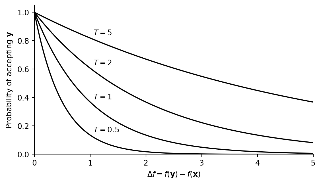
Figure 30.3 shows the length of the current tour \mathbf{x} at each iteration. While the temperature is high, many exchanges that lengthen the tour are accepted, and the tour length goes up and down. As the temperature decreases, fewer exchanges that lengthen the tour are accepted. The search then behaves like local search.

Code
from matplotlib.ticker import StrMethodFormatter

fig, ax = plt.subplots(figsize=(6, 3.5))
ax.plot(lengths_sa, color="black", linewidth=0.5)
ax.axhline(optimal_length, color="black", linestyle=":", linewidth=1)
ax.text(0, optimal_length, "Optimal", va="bottom")
ax.set_ylim(10_500, 21_000)
ax.set_xlabel("Iteration")
ax.set_ylabel("Tour length (miles)")
ax.xaxis.set_major_formatter(StrMethodFormatter("{x:,.0f}"))
ax.yaxis.set_major_formatter(StrMethodFormatter("{x:,.0f}"))

# The k-th temperature T0 * gamma**k (k = 0, 1, ...) is used from iteration k * L,
# so T is reached after about L * log(T / T0) / log(gamma) iterations
temperatures = [300, 100, 30, 10, 3]
temperature_axis = ax.secondary_xaxis("top")
temperature_axis.set_xticks(
    [L * np.log(T / T0) / np.log(gamma) for T in temperatures],
    labels=[str(T) for T in temperatures],
)
temperature_axis.set_xlabel("Temperature $T$")
fig.tight_layout()
plt.show()
Line chart of the length of the current tour in miles against iteration, from 0 to 49,500, with a second horizontal axis at the top showing the temperature: 300 at iteration 0, 100 near iteration 10,600, 30 near 22,200, 10 near 32,800, and 3 near 44,400. The vertical axis runs from 10,500 to 21,000 miles, so the start of the line at 42,650 miles is cut off. Between iterations 500 and 10,000, the line goes up and down between about 11,100 and 20,200 miles. The swings shrink as the temperature falls. The line first touches the dotted line of the optimal length, 10,861 miles, near iteration 17,000, rises above it again, and stays on it from about iteration 30,700 to the end.
Figure 30.3: Length of the current tour at each iteration of simulated annealing, starting from the initial tour in Figure 29.2. The upper axis shows the temperature T. The initial tour (42,650 miles) lies above the plotted range.

Simulated annealing makes random choices, so another run may return a different tour. The following code runs simulated annealing and first-improvement local search from the same 100 random initial tours.

n_runs = 100
rng = np.random.default_rng(0)
sa_lengths, final_lengths, ls_lengths = [], [], []
for _ in range(n_runs):
    random_tour = rng.permutation(n).tolist()
    best_tour, lengths = simulated_annealing(
        random_tour, D, T0, gamma, L, n_iterations, rng
    )
    sa_lengths.append(tour_length(best_tour, D))
    final_lengths.append(lengths[-1])
    _, lengths = local_search(random_tour, D, first_improvement)
    ls_lengths.append(lengths[-1])

for name, results in [
    ("Simulated annealing", sa_lengths),
    ("Local search", ls_lengths),
]:
    print(
        f"{name:20} optimal in {results.count(optimal_length):2} runs, "
        f"average {np.mean(results):,.0f} miles"
    )
Simulated annealing  optimal in 35 runs, average 10,938 miles
Local search         optimal in 12 runs, average 11,190 miles

Simulated annealing returns an optimal tour in 35 of the 100 runs, compared with 12 for local search, and its average length is shorter (10,938 versus 11,190 miles). However, each run of simulated annealing evaluates 49,500 neighbors, whereas local search stops as soon as it reaches a local optimum.