9  Branch and Bound

The branch and bound is an algorithm for solving combinatorial optimization problems exactly by intelligently exploring the solution space.

The branch refers to the process of partitioning the solution space. The bound refers to lower bounds that are used to construct a proof of optimality.

One of the important applications of branch and bound is the Integer Programming (IP) problem. Furthermore, branch and bound is also an idea that can be applied to almost any optimization problem with combinatorial nature. We will first introduce the branch and bound algorithm for the IP problem, and then we illustrate the general branch and bound algorithm.

9.1 Branch and Bound for IP Problem

Consider the following integer programming problem:

\begin{aligned} (P_0) \qquad \min \quad & \mathbf{c}^{\top} \mathbf{x} \\ \text{s.t.} \quad & \mathbf{A} \mathbf{x} \leq \mathbf{b} \\ & \mathbf{x} \geq 0 \\ & \mathbf{x} \in \mathbb{Z}^{n} \end{aligned}

The LP relaxation of an IP problem is obtained by removing the integrality constraints. The LP relaxation of P_0 is given by

\begin{aligned} \min \quad & \mathbf{c}^{\top} \mathbf{x} \\ \text{s.t.} \quad & \mathbf{A} \mathbf{x} \leq \mathbf{b} \\ & \mathbf{x} \geq 0 \end{aligned}

Solving this LP relaxation problem gives a solution \mathbf{x}^0 and an optimal value z^0 = \mathbf{c}^{\top} \mathbf{x}^0. Since every feasible solution to the original IP problem is also feasible for the LP relaxation, z^0 is a lower bound of the original IP problem. That is, the optimal value of the original IP problem must be larger than or equal to z^0. If \mathbf{x}^0 is an integer solution, then it is also the optimal solution to the original IP problem.

Otherwise, we choose a variable x_i whose value x_i^0 is not an integer, and generate two new subproblems by adding the constraints x_i \leq \lfloor x_i^0 \rfloor and x_i \geq \lceil x_i^0 \rceil, respectively. Here, \lfloor x \rfloor and \lceil x \rceil are the floor and ceiling functions, respectively. Later, we will discuss how to choose the variable x_i. As a result, we have two subproblems:

\begin{aligned} (P_1) \qquad \min \quad & \mathbf{c}^{\top} \mathbf{x} \\ \text{s.t.} \quad & \mathbf{A} \mathbf{x} \leq \mathbf{b} \\ & x_i \leq \lfloor x_i^0 \rfloor \\ & \mathbf{x} \geq 0 \\ & \mathbf{x} \in \mathbb{Z}^{n} \end{aligned}

and

\begin{aligned} (P_2) \qquad \min \quad & \mathbf{c}^{\top} \mathbf{x} \\ \text{s.t.} \quad & \mathbf{A} \mathbf{x} \leq \mathbf{b} \\ & x_i \geq \lceil x_i^0 \rceil \\ & \mathbf{x} \geq 0 \\ & \mathbf{x} \in \mathbb{Z}^{n} \end{aligned}

Since x_i must be an integer, every feasible solution to the original IP problem satisfies one of the constraints, x_i \leq \lfloor x_i^0 \rfloor or x_i \geq \lceil x_i^0 \rceil, while \mathbf{x}^0 satisfies neither of them. Therefore, now we can find the optimal solution to the original IP problem by solving these two subproblems.

Say we solve the LP relaxation of P_1 and obtain a solution \mathbf{x}^1 and an optimal value z^1 = \mathbf{c}^{\top} \mathbf{x}^1. If \mathbf{x}^1 is an integer solution, then it is a feasible solution to the original IP problem, and z^1 is an upper bound on the optimal value. It is not necessarily optimal, because P_2 may contain a better solution. Otherwise, z^1 is a lower bound for P_1, and we can generate two new subproblems by adding constraints.

We can repeat this process for P_2 as well. In general, we number the subproblems P_1, P_2, \dots in the order they are generated, and for each subproblem P_k, let \mathbf{x}^k and z^k = \mathbf{c}^{\top} \mathbf{x}^k be the optimal solution and the optimal value of its LP relaxation. In the searching process, the LP relaxations of some subproblems may have an optimal integer solution. These allow us to keep track of the upper bound. Every time we find a new integer solution with the lowest objective value, we update the upper bound. With the upper bound, we can prune some subproblems.

Say the LP relaxation of a subproblem P_k has an integer solution \mathbf{x}^k. When z^k is the lowest among all integer solutions found so far, we let z^k be the current upper bound. If a subproblem P_j has a lower bound z^j \geq z^k, then we do not need to further branch on P_j, because it cannot contain a better solution than the current best solution. We say that this subproblem is pruned.

In general, we can keep branching on subproblems until (1) we find an integer solution, or (2) the solution is infeasible, or (3) the lower bound of a subproblem is larger than or equal to the current upper bound.

This process can be represented as a tree, where each node represents a subproblem. The root node is the original IP problem P_0, and the children of a node are the two subproblems generated by branching on a variable.

Example 9.1 (A two-variable IP problem) Consider the following IP problem:

\begin{aligned} (P_0) \qquad \min \quad & 5x_1 + 3x_2 \\ \text{s.t.} \quad & 4x_1 + x_2 \geq 8 \\ & 2x_1 + 2x_2 \geq 7 \\ & x_1, x_2 \geq 0 \\ & x_1, x_2 \in \mathbb{Z} \end{aligned}

We use the notation P_k, \mathbf{x}^k, and z^k introduced above.

Figure 9.1 shows the searching process of branch and bound as a tree.

Code
import matplotlib.pyplot as plt

# Subproblem k: position in the tree, and the optimal solution x^k and the
# optimal value z^k of its LP relaxation
nodes = {
    0: dict(pos=(1.125, 3), x=(1.5, 2), z=13.5),
    1: dict(pos=(0, 2), x=(1, 4), z=17, note="integer"),
    2: dict(pos=(2.25, 2), x=(2, 1.5), z=14.5),
    3: dict(pos=(1.5, 1), x=(2.5, 1), z=15.5),
    4: dict(pos=(3, 1), x=(2, 2), z=16, note="integer, optimal"),
    5: dict(pos=(1, 0)),  # infeasible
    6: dict(pos=(2, 0), x=(3, 0.5), z=16.5, note="pruned by bound"),
}
discarded = {5, 6}  # gray boxes
optimal = 4  # thick box
# Parent, child, and the constraint added by branching
edges = [
    (0, 1, r"$x_1 \leq 1$"),
    (0, 2, r"$x_1 \geq 2$"),
    (2, 3, r"$x_2 \leq 1$"),
    (2, 4, r"$x_2 \geq 2$"),
    (3, 5, r"$x_1 \leq 2$"),
    (3, 6, r"$x_1 \geq 3$"),
]

# Computer Modern fonts, as in LaTeX. The last setting avoids a warning about cmr10.
latex_style = {
    "font.family": "cmr10",
    "mathtext.fontset": "cm",
    "axes.formatter.use_mathtext": True,
}
with plt.rc_context(latex_style):
    fig, ax = plt.subplots(figsize=(6.5, 4.6))
    for parent, child, label in edges:
        (px, py), (cx, cy) = nodes[parent]["pos"], nodes[child]["pos"]
        ax.plot([px, cx], [py, cy], color="black", linewidth=1, zorder=1)
        # Place the label on the outer side of the edge
        side = 1 if cx > px else -1
        ax.text(
            (px + cx) / 2 + 0.07 * side,
            (py + cy) / 2,
            label,
            ha="left" if side > 0 else "right",
            va="center",
            fontsize=11,
        )

    for k, node in nodes.items():
        if "x" in node:
            lines = [
                rf"$P_{k}$",
                rf"$\mathbf{{x}} = ({node['x'][0]:g},\, {node['x'][1]:g})$",
                rf"$z = {node['z']:g}$",
            ]
        else:
            lines = [rf"$P_{k}$", "infeasible"]
        ax.text(
            *node["pos"],
            "\n".join(lines),
            ha="center",
            va="center",
            fontsize=11,
            linespacing=1.4,
            zorder=2,
            bbox=dict(
                boxstyle="square,pad=0.4",
                facecolor="lightgray" if k in discarded else "white",
                edgecolor="black",
                linewidth=2 if k == optimal else 1,
            ),
        )
        if "note" in node:
            pos = node["pos"]
            ax.text(
                pos[0],
                pos[1] - 0.4,
                node["note"],
                ha="center",
                va="top",
                fontsize=10,
                color="dimgray",
            )

    ax.set(xlim=(-0.5, 3.5), ylim=(-0.7, 3.35))
    ax.axis("off")
    fig.subplots_adjust(left=0, right=1, top=1, bottom=0)
    plt.show()
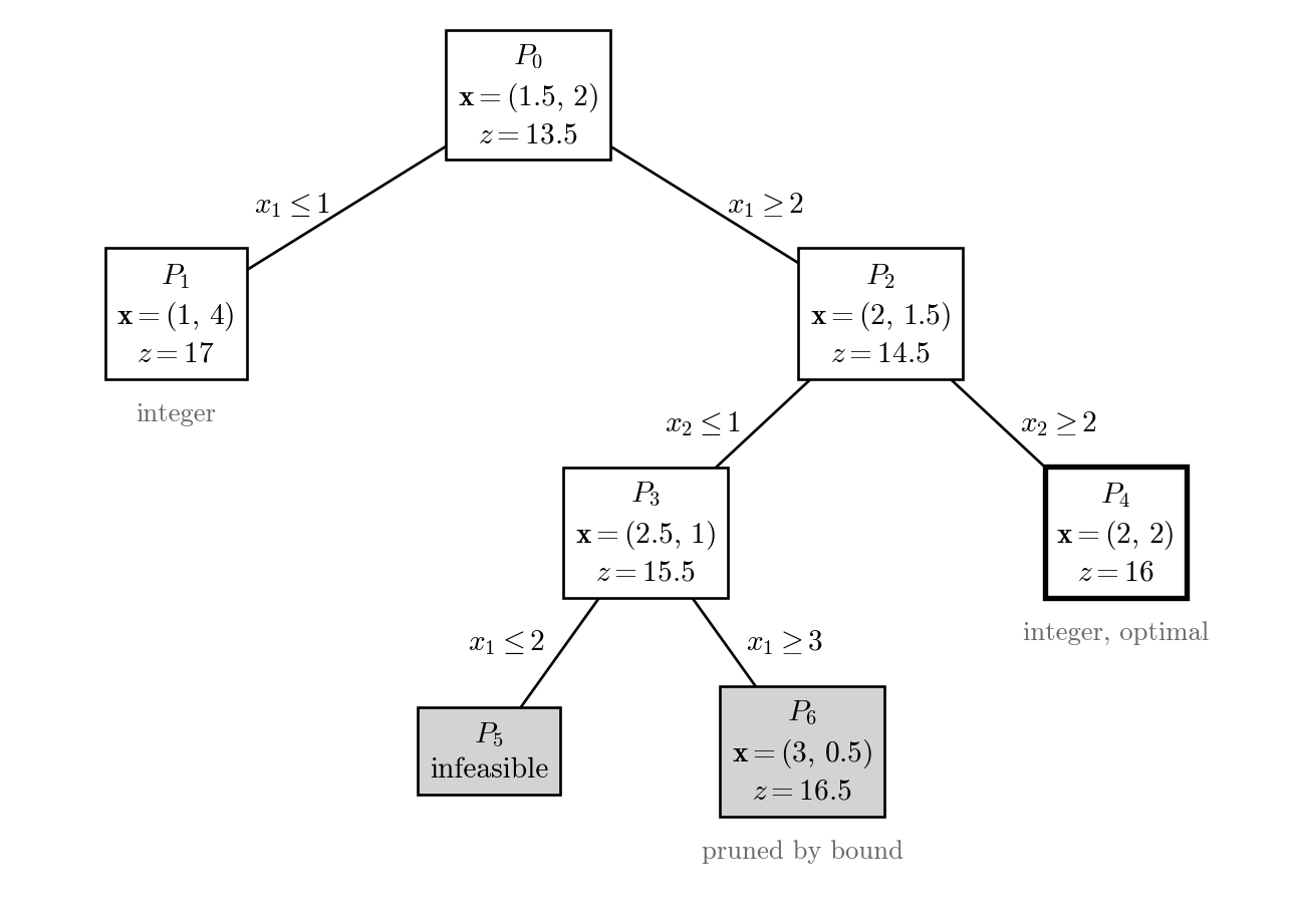
A tree of seven boxes, P0 to P6, connected by lines and drawn in black, white, and gray. The root P0 at the top has x = (1.5, 2) and z = 13.5. The branch x1 ≤ 1 leads to P1 with x = (1, 4) and z = 17, labeled integer. The branch x1 ≥ 2 leads to P2 with x = (2, 1.5) and z = 14.5. From P2, the branch x2 ≤ 1 leads to P3 with x = (2.5, 1) and z = 15.5, and the branch x2 ≥ 2 leads to P4 with x = (2, 2) and z = 16, which has a thick border and is labeled integer, optimal. From P3, the branch x1 ≤ 2 leads to the gray box P5, labeled infeasible, and the branch x1 ≥ 3 leads to the gray box P6 with x = (3, 0.5) and z = 16.5, labeled pruned by bound.
Figure 9.1: Branch-and-bound tree. Each box shows a subproblem with the optimal solution \mathbf{x} and the optimal value z of its LP relaxation, and each edge shows the constraint added by branching. Gray boxes are infeasible or pruned by bound, and the thick box gives the optimal solution.

Note that P_5 is infeasible. It has the constraints x_1 \geq 2 from P_2, x_2 \leq 1 from P_3, and x_1 \leq 2. Thus x_1 = 2, and 2x_1 + 2x_2 \geq 7 requires x_2 \geq 1.5, which contradicts x_2 \leq 1. For P_6, \mathbf{x}^6 = (3, 0.5) and z^6 = 16.5.

We do not need to branch on P_6 because its lower bound z^6 = 16.5 is larger than the upper bound z^4 = 16 from P_4.

Therefore, \mathbf{x}^4 = (2, 2) is an optimal solution, and the optimal value is 16.

To implement the branch and bound algorithm for the IP problem, there are two more important issues to consider: (1) how to choose the variable x_i to branch on, and (2) how to choose the next subproblem to branch on.

9.1.1 Choosing the Branching Variable

If the LP solution \mathbf{x}^k of a subproblem P_k has more than one variable whose value is not an integer, we can branch on any of them. (In Example 9.1, there was always only one such variable.) Any choice leads to an optimal solution, but the number of subproblems we have to solve can change greatly. Two simple rules are as follows.

  • Most fractional branching: Choose the variable whose fractional part x_i^k - \lfloor x_i^k \rfloor is closest to 0.5. This rule is easy to implement, but it does not consider how much the objective value changes after branching.
  • Strong branching: For each variable x_i whose value x_i^k is not an integer, solve the LP relaxations of the two subproblems with x_i \leq \lfloor x_i^k \rfloor and x_i \geq \lceil x_i^k \rceil. If an LP relaxation is infeasible, we regard its optimal value as \infty. Every feasible solution to P_k is feasible for one of the two new subproblems, so the smaller of the two optimal values is a lower bound for P_k. Choose the variable that makes this lower bound the largest. Strong branching usually gives a much smaller tree than most fractional branching, but each branching requires solving two LPs for every such variable.

9.1.2 Choosing the Next Subproblem

During the search, we keep a list of subproblems that are waiting to be explored, and we can choose any of them next. Two basic rules are as follows.

  • Depth-first search: Choose the subproblem that was generated most recently. The search goes down the tree until it cannot branch any more, and then goes back up. Integer solutions are usually found deep in the tree, so depth-first search tends to find an upper bound early. It also keeps only a few subproblems at a time.
  • Best-first search: Choose the subproblem with the smallest lower bound, that is, the most promising one. It tends to solve fewer subproblems than depth-first search. However, it may keep many subproblems at a time, and it may take a long time to find the first integer solution.
NoteResearch on branching rules and node selection

In the literature, a rule for choosing the branching variable is called a branching rule, and choosing the next subproblem is called node selection.

Computational studies show that most fractional branching (also called most infeasible branching) is on average no better than choosing a variable at random, and that strong branching gives by far the smallest trees but takes too much time (Achterberg et al. 2005). Pseudocost branching (Benichou et al. 1971) estimates the increase of the lower bound from the branchings performed earlier in the search. It is fast, but it has no information at the beginning of the search. Reliability branching (Achterberg et al. 2005) combines the two: it uses strong branching only for the variables whose estimates are not yet reliable. A variant of reliability branching is the default branching rule of the solver SCIP (Achterberg 2007, chap. 5).

If the branching rule is fixed and ties are broken appropriately, best-first search branches on the fewest subproblems, because a subproblem whose lower bound is smaller than the optimal value can never be pruned (Fox et al. 1978; Achterberg 2007, sec. 6.2). To also find integer solutions early, solvers often combine the two rules: the search goes down the tree as in depth-first search for a while, and then jumps to a subproblem with a small lower bound (Achterberg 2007, chap. 6). Linderoth and Savelsbergh (1999) compare many branching rules and node selection rules computationally.

No rule is the best for all problems, and recent research uses machine learning to learn these rules from data (Lodi and Zarpellon 2017; Scavuzzo et al. 2024). For a survey of branch-and-bound algorithms, see Morrison et al. (2016).

Depth-first search keeps the waiting subproblems in a stack, and best-first search keeps them in a priority queue. These data structures and their Python classes queue.LifoQueue and queue.PriorityQueue are introduced in Section 7.2.

Example 9.2 (Subproblems in a priority queue) For best-first search, the key of a subproblem P_k is its lower bound z^k, so we put the tuple (z^k, k) into the priority queue. Python compares two tuples by their first elements, and by their second elements only if the first elements are equal. The following code adds P_1, P_2, P_3, and P_4 with z^1 = 5, z^2 = 2, z^3 = 7, and z^4 = 3 in this order.

from queue import PriorityQueue

priority_queue = PriorityQueue()
priority_queue.put((5, 1))
priority_queue.put((2, 2))
priority_queue.put((7, 3))
priority_queue.put((3, 4))
print(priority_queue.get())
(2, 2)
(3, 4)
(5, 1)
(7, 3)

The priority queue takes the subproblems out in increasing order of z^k: P_2, P_4, P_1, and P_3.

Example 9.3 (A 0-1 knapsack problem) Consider the following 0-1 knapsack problem with four items:

\begin{aligned} (P_0) \qquad \max \quad & \mathbf{c}^{\top} \mathbf{x} \\ \text{s.t.} \quad & \mathbf{w}^{\top} \mathbf{x} \leq C \\ & \mathbf{x} \in \{0, 1\}^{4} \end{aligned}

where \mathbf{c} = (9, 6, 11, 4) and \mathbf{w} = (1, 2, 4, 4). Here x_i = 1 means that item i is put into the knapsack. Item i has a value c_i and a weight w_i, and the capacity of the knapsack is set to C = 6.

Table 9.1 lists them together with the value per unit weight c_i / w_i, which we use below.

Table 9.1: Items of the knapsack problem (capacity 6)
Item i Value c_i Weight w_i c_i / w_i
1 9 1 9
2 6 2 3
3 11 4 2.75
4 4 4 1

The LP relaxation replaces x_i \in \{0, 1\} with 0 \leq x_i \leq 1, so a fraction of an item can be put into the knapsack. We can solve it by a greedy method:

  1. put the items into the knapsack in decreasing order of the value per unit weight c_i / w_i, and
  2. when an item does not fit, put only the fraction of it that fills the knapsack, and stop.

This works because each unit of capacity should be used for the remaining item with the largest c_i / w_i. In Table 9.1, the items are already in this order. Items 1 and 2 use a capacity of 3, and 3/4 of item 3 fills the remaining capacity 3. Thus \mathbf{x}^0 = (1, 1, 0.75, 0) and z^0 = 9 + 6 + 11 \times 0.75 = 23.25.

Since this is a maximization problem, the roles of the bounds are reversed: z^k is an upper bound for P_k, and an integer solution gives a lower bound on the optimal value. Thus P_k is pruned if z^k is less than or equal to the value of the best integer solution found so far.

The solution of the greedy method has at most one fractional variable x_i, so we branch on this variable; both branching rules above choose it. Since x_i \in \{0, 1\}, the constraints x_i \leq \lfloor x_i^k \rfloor and x_i \geq \lceil x_i^k \rceil become x_i = 0 and x_i = 1. To solve the LP relaxation of a subproblem, we first put the items with x_i = 1 into the knapsack, and then apply the greedy method to the items that are not fixed. If the items with x_i = 1 do not fit, the subproblem is infeasible.

We choose the next subproblem by depth-first search. When we branch on x_i, we generate the subproblem with x_i = 0 first and the one with x_i = 1 next, so depth-first search goes to the side with x_i = 1 first.

Figure 9.2 shows the tree.

Code
import matplotlib.pyplot as plt

# Subproblem k: position in the tree, and the optimal solution x^k and the
# optimal value z^k of its LP relaxation, found by the greedy method
nodes = {
    0: dict(pos=(1.125, 3), x=(1, 1, 0.75, 0), z=23.25),
    1: dict(pos=(0, 2), x=(1, 1, 0, 0.75), z=18, note="pruned by bound"),
    2: dict(pos=(2.25, 2), x=(1, 0.5, 1, 0), z=23),
    3: dict(pos=(1.5, 1), x=(1, 0, 1, 0.25), z=21),
    4: dict(pos=(3, 1), x=(0, 1, 1, 0), z=17, note="integer"),
    5: dict(pos=(1, 0), x=(1, 0, 1, 0), z=20, note="integer, optimal"),
    6: dict(pos=(2, 0)),  # infeasible
}
discarded = {1, 6}  # gray boxes
optimal = 5  # thick box
# Parent, child, and the variable fixed by branching
edges = [
    (0, 1, r"$x_3 = 0$"),
    (0, 2, r"$x_3 = 1$"),
    (2, 3, r"$x_2 = 0$"),
    (2, 4, r"$x_2 = 1$"),
    (3, 5, r"$x_4 = 0$"),
    (3, 6, r"$x_4 = 1$"),
]

# Computer Modern fonts, as in LaTeX. The last setting avoids a warning about cmr10.
latex_style = {
    "font.family": "cmr10",
    "mathtext.fontset": "cm",
    "axes.formatter.use_mathtext": True,
}
with plt.rc_context(latex_style):
    fig, ax = plt.subplots(figsize=(6.5, 4.6))
    for parent, child, label in edges:
        (px, py), (cx, cy) = nodes[parent]["pos"], nodes[child]["pos"]
        ax.plot([px, cx], [py, cy], color="black", linewidth=1, zorder=1)
        # Place the label on the outer side of the edge
        side = 1 if cx > px else -1
        ax.text(
            (px + cx) / 2 + 0.07 * side,
            (py + cy) / 2,
            label,
            ha="left" if side > 0 else "right",
            va="center",
            fontsize=11,
        )

    for k, node in nodes.items():
        if "x" in node:
            x = r",\, ".join(f"{v:g}" for v in node["x"])
            lines = [
                rf"$P_{k}$",
                rf"$\mathbf{{x}} = ({x})$",
                rf"$z = {node['z']:g}$",
            ]
        else:
            lines = [rf"$P_{k}$", "infeasible"]
        ax.text(
            *node["pos"],
            "\n".join(lines),
            ha="center",
            va="center",
            fontsize=11,
            linespacing=1.4,
            zorder=2,
            bbox=dict(
                boxstyle="square,pad=0.4",
                facecolor="lightgray" if k in discarded else "white",
                edgecolor="black",
                linewidth=2 if k == optimal else 1,
            ),
        )
        if "note" in node:
            pos = node["pos"]
            ax.text(
                pos[0],
                pos[1] - 0.4,
                node["note"],
                ha="center",
                va="top",
                fontsize=10,
                color="dimgray",
            )

    ax.set(xlim=(-0.5, 3.5), ylim=(-0.7, 3.35))
    ax.axis("off")
    fig.subplots_adjust(left=0, right=1, top=1, bottom=0)
    plt.show()
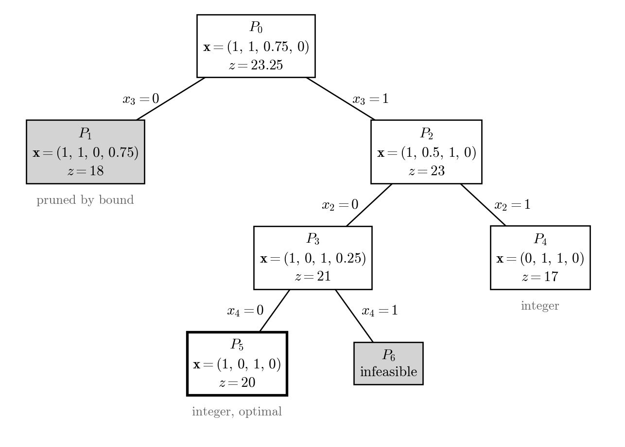
A tree of seven boxes, P0 to P6, connected by lines and drawn in black, white, and gray. The root P0 at the top has x = (1, 1, 0.75, 0) and z = 23.25. The branch x3 = 0 leads to the gray box P1 with x = (1, 1, 0, 0.75) and z = 18, labeled pruned by bound. The branch x3 = 1 leads to P2 with x = (1, 0.5, 1, 0) and z = 23. From P2, the branch x2 = 0 leads to P3 with x = (1, 0, 1, 0.25) and z = 21, and the branch x2 = 1 leads to P4 with x = (0, 1, 1, 0) and z = 17, labeled integer. From P3, the branch x4 = 0 leads to P5 with x = (1, 0, 1, 0) and z = 20, which has a thick border and is labeled integer, optimal, and the branch x4 = 1 leads to the gray box P6, labeled infeasible.
Figure 9.2: Branch-and-bound tree for the knapsack problem. Each box shows a subproblem with the optimal solution \mathbf{x} and the optimal value z of its LP relaxation, and each edge shows the variable fixed by branching. Gray boxes are infeasible or pruned by bound, and the thick box gives the optimal solution. Depth-first search chooses the subproblems in the order P_0, P_2, P_3, P_1.

The search proceeds as follows.

  1. We branch on x_3 in P_0. In P_2, item 3 uses a capacity of 4, and the greedy method puts item 1 and half of item 2 into the remaining capacity 2.
  2. P_2 was generated last, so we choose it and branch on x_2. In P_4, items 2 and 3 fill the knapsack, so \mathbf{x}^4 = (0, 1, 1, 0) is an integer solution. The lower bound is now z^4 = 17.
  3. The waiting subproblems are P_1 and P_3, and P_3 was generated last. Since z^3 = 21 > 17, we branch on x_4. \mathbf{x}^5 = (1, 0, 1, 0) is an integer solution with z^5 = 20 > 17, so the lower bound is updated to 20. P_6 is infeasible, because items 3 and 4 have a total weight of 8 > 6.
  4. Only P_1 is left. Since z^1 = 18 \leq 20, P_1 is pruned.

No subproblem is left. Therefore, \mathbf{x}^5 = (1, 0, 1, 0) is an optimal solution, and the optimal value is 20. Note that rounding down \mathbf{x}^0 gives (1, 1, 0, 0) with value 15, which is not optimal.

9.2 General Branch-and-Bound Algorithm

\begin{algorithm} \caption{General Branch-and-Bound Algorithm} \begin{algorithmic} \Procedure{BranchAndBound}{} \State Initialize current best node $v^*$ \State UB $\gets \infty$ \State Create a queue $Q$ \State $Q.\text{put}(root)$ \While{$Q$ is not empty} \State $k \gets Q.\text{get}()$ \State generate children of node $k$, child $i \in \mathcal{S}(k)$ \State generate lower bounds $LB_i$ for each child $i$ \For{each $i \in \mathcal{S}(k)$} \If{$LB_i \geq$ UB} \State kill child $i$ \ElsIf{child $i$ is a leaf node} \State UB $\gets$ value of child $i$ \State $v^* \gets i$ \Else \State $Q.\text{put}(i)$ \EndIf \EndFor \EndWhile \EndProcedure \end{algorithmic} \end{algorithm}

9.3 Example: Shortest Path Problem

Branch and Bound algorithm for the shortest path problem

We branch from a node with the lowest lower bound using a priority queue.

from queue import PriorityQueue
import networkx as nx

# shortest path problem
class ShortestPathProblem:
    def __init__(self, graph):
        self.graph = graph
    
    def branch(self, node):
        children = []
        weights = []
        # Generate children of the node
        for child in self.graph.successors(node):
            children.append(child)
            weights.append(self.graph[node][child]['weight'])

        return children, weights

# Node class in the branch and bound algorithm
class Node:
    def __init__(self, node_idx, lower_bound):
        self.node_idx = node_idx
        self.lower_bound = lower_bound
        self.solution = []

    def update_solution(self, parent_solution):
        self.solution = parent_solution.copy()
        self.solution.append(self.node_idx)

    def __lt__(self, other):
        return self.lower_bound < other.lower_bound

def branch_and_bound(problem):
    
    U = float('inf')
    current_best_solution = None
    current_best_value = None

    priority_queue = PriorityQueue(maxsize=0)

    # Initialize the priority queue with the root node
    root_node = Node(0, 0)
    root_node.solution.append(0)
    priority_queue.put((0, root_node))

    while not priority_queue.empty():

        _, node = priority_queue.get()

        # generate children of the node
        children, weights = problem.branch(node.node_idx)

        for child, weight in zip(children, weights):
            z = node.lower_bound + weight

            if z >= U:
                continue
            elif child == 10:
                U = z
                current_best_value = z
                current_best_solution = node.solution.copy()
            else:
                new_node = Node(child, z)
                new_node.update_solution(node.solution)
                priority_queue.put((z, new_node))

    return current_best_value, current_best_solution


if __name__ == '__main__':

    '''
    Define the shortest-path problem.
    Example from the book:
    Papadimitriou, Christos H., and Kenneth Steiglitz. 1998. Combinatorial Optimization: Algorithms and Complexity. Courier Corporation.    
    '''
    G = nx.DiGraph()

    # Add nodes
    G.add_nodes_from(range(0, 11))

    # Add edges
    G.add_edge(0, 1, weight=2)
    G.add_edge(0, 2, weight=3)
    G.add_edge(0, 3, weight=4)
    G.add_edge(1, 4, weight=7)
    G.add_edge(1, 5, weight=2)
    G.add_edge(1, 2, weight=3)
    G.add_edge(2, 5, weight=9)
    G.add_edge(2, 6, weight=2)
    G.add_edge(3, 6, weight=2)
    G.add_edge(4, 7, weight=1)
    G.add_edge(4, 8, weight=2)
    G.add_edge(5, 8, weight=3)
    G.add_edge(5, 6, weight=1)
    G.add_edge(6, 8, weight=5)
    G.add_edge(6, 9, weight=1)
    G.add_edge(7, 10, weight=4)
    G.add_edge(8, 10, weight=4)
    G.add_edge(9, 10, weight=2)
    G.add_edge(9, 8, weight=2)

    spp = ShortestPathProblem(G)


    value, solution = branch_and_bound(spp)
    print('Shortest path value:', value)
    print('Shortest path:', solution)