14  経済的発注量

14.1 学習目標

• EOQモデルの仮定と，最適解がもつ2つの性質を理解する．
• 平均コスト関数 g(Q) を導出できる．
• EOQ公式を導出し，最適発注量と最適サイクル期間を求めることができる．
• パラメータの変化が最適発注量に与える影響を説明できる．
• *リードタイムがある場合の発注点を求めることができる．

14.2 前提知識

• 数学：微分積分
• 在庫の費用と在庫方策：チャプター 13

14.3 EOQモデルとは

経済的発注量（EOQ: Economic Order Quantity）モデルは，最も基本的な在庫管理モデルの一つである．Harris (1990年) がこのモデルを最初に提案した．

EOQモデルは，次の4つの仮定をおく．

1. 需要は決定論的で一定である． 単位時間あたりの需要量は事前に分かっており，時間とともに変化しない．この需要量を需要率（demand rate）と呼び，d で表す．
2. リードタイムは0である． 発注から納品までに時間はかからない．
3. 欠品は許さない． すべての需要は在庫から満たされなければならない．
4. 在庫量は連続的に観測され，いつでも発注できる．

在庫に関わる費用には，1回あたりの発注費用 K，単位時間あたりの1単位の保管費用 h，購入単価 c がある（チャプター 13）．

これらの仮定のもとで，EOQモデルの最適解は次の二つの性質を持つ(Snyder と Shen 2019年)．

1. Zero-inventory ordering (ZIO)：在庫量が0のときに発注を行う．リードタイムは0であるため，在庫量が0でないときに発注すると，保管費用が余分に発生する．
2. Constant order sizes：発注量は一定である．需要率 d が一定であり，かつ在庫量が0のときに発注するため，どのサイクルも同じ状況から始まるからである．

以降では，この2つの性質を満たす方策のみを考え，1回あたりの発注量を Q と書く．

14.4 記号

記号	意味
d	単位時間あたりの需要量
K	1回あたりの発注費用
h	単位時間あたりの1単位の保管費用
c	購入単価
Q	発注量
T	サイクル期間
g(Q)	平均コスト

14.5 サイクル

発注の間隔をサイクル（cycle）と呼び，サイクル期間は

T = \frac{Q}{d}

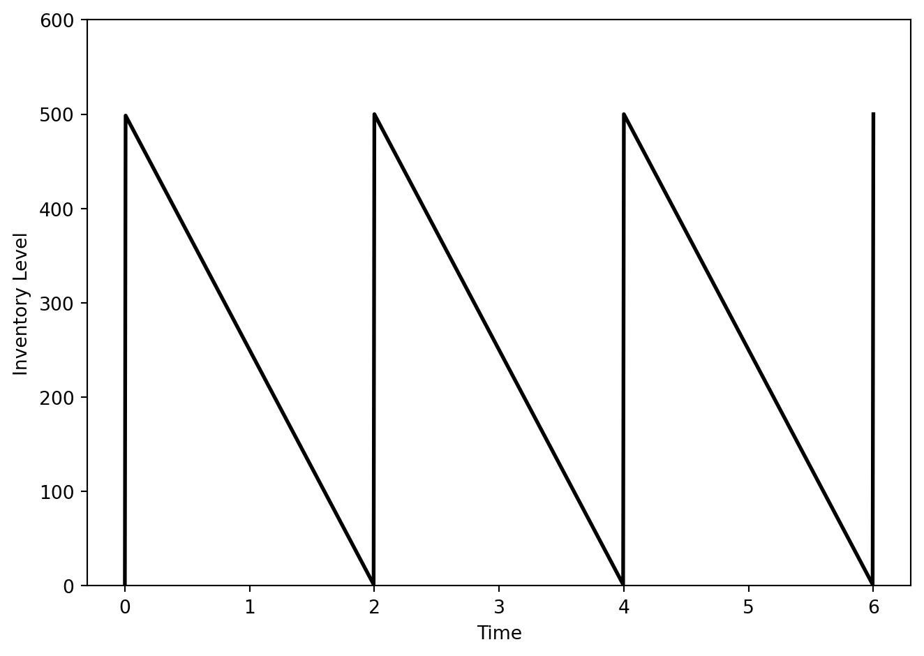
で与えられる．ZIOと発注量一定の2つの性質から，在庫量の時間的変化は 図 14.1 のような鋸歯状になる．在庫量は発注直後に Q となり，需要率 d で直線的に減少し，0になった時点で次の発注が届く．

import matplotlib.pyplot as plt

# Parameters
d = 250  # Demand rate
Q = 500  # Order quantity
T = Q / d  # Cycle length
n_cycles = 3

# Inventory level over time: each cycle falls from Q to 0 at rate d,
# then the next order arrives instantaneously.
t = [0.0]
inventory = [Q]
for i in range(n_cycles):
    t += [(i + 1) * T, (i + 1) * T]
    inventory += [0, Q]
t, inventory = t[:-1], inventory[:-1]  # drop the trailing jump back to Q

# Plotting the inventory level
plt.plot(t, inventory, color="#16212d", linewidth=2)  # brand: ink
plt.axhline(Q / 2, color="#5b6b7c", linestyle="--", linewidth=1)  # brand: slate
plt.xlabel("Time")
plt.ylabel("Inventory Level")
plt.xticks([i * T for i in range(n_cycles + 1)], ["$0$", "$T$", "$2T$", "$3T$"])
plt.yticks([0, Q / 2, Q], ["$0$", "$Q/2$", "$Q$"])
plt.xlim(0, n_cycles * T)
plt.ylim(0, Q * 1.15)
plt.tight_layout()
plt.show()

図 14.1: EOQモデルにおける在庫量の時間的変化

例 14.1 A社は，毎月250個の需要がある商品を取り扱っている．1回の発注量は500個とし，サイクル期間は

T = \frac{500}{250} = 2 \text{ヶ月}

となる．

14.6 コスト関数

どのサイクルも同じ状況から始まるため，コストはサイクルごとに繰り返される．そこでまず1サイクルあたりのコストを求め，それをサイクル期間で割って単位時間あたりの平均コストを得る．

発注費用：1サイクルに発注は1回だけであるため，発注費用は K である．

購入費用：Q 個の商品を単価 c で購入するため，購入費用は cQ である．

保管費用：在庫量は Q から0まで直線的に減少するため，サイクル中の平均在庫量は \frac{Q}{2} である．これが期間 T = \frac{Q}{d} にわたって保管されるため，1サイクルあたりの保管費用は

h \cdot \frac{Q}{2} \cdot T = \frac{hQ^2}{2d}

となる．

以上より，1サイクルあたりのコストは次のように表される．

K + cQ + \frac{hQ^2}{2d}

平均コストは，これをサイクル期間 T で割ったものとして定義される．\frac{1}{T} = \frac{d}{Q} であるから，

\begin{align*} g(Q) &= \frac{1}{T} \left( K + cQ + \frac{hQ^2}{2d} \right) \\ &= \frac{d}{Q} \left( K + cQ + \frac{hQ^2}{2d} \right) \\ &= \frac{Kd}{Q} + c d + \frac{hQ}{2} \end{align*}

となる．すなわち，平均コストは発注量 Q の関数として

g(Q) = \frac{Kd}{Q} + cd + \frac{hQ}{2} \tag{14.1}

と表される．第1項 \frac{Kd}{Q} を発注コスト，第3項 \frac{hQ}{2} を保管コストと呼ぶ．いずれも単位時間あたりの平均である．

14.7 最適発注量

EOQモデルの目的は，平均コスト g(Q) を最小化する発注量 Q を求めることである．式 14.1 の第1項は Q について減少し，第3項は増加するため，両者を釣り合わせる Q が存在する．

そこで，導関数 g'(Q) が 0 となる点を求める．

g'(Q) = -\frac{Kd}{Q^2} + \frac{h}{2} = 0

これを解くと，最適発注量

Q^* = \sqrt{\frac{2Kd}{h}}

を得る．これをEOQ公式（EOQ formula）と呼び，Q^* が冒頭の経済的発注量である（ここでの「経済的」は最適という意味である）．

Q^* が最小値を与えることを，二階導関数 g''(Q) で確認する．

g''(Q) = \frac{2Kd}{Q^3} > 0

g''(Q) > 0 であるため，Q^* は最小値を与える．

最適発注量 Q^* を次の定理にまとめる．

定理 14.1 EOQモデルにおいて，最適発注量 Q^* は Q^* = \sqrt{\frac{2Kd}{h}} \tag{14.2}

で与えられる．

Q^* を用いると，最適なサイクル期間 T^* は次のように求められる．

T^* = \frac{Q^*}{d} = \sqrt{\frac{2K}{hd}} \tag{14.3}

式 14.2 と 式 14.3 から，以下の性質がわかる．

1. h の増加に伴い，Q^* は減少する．保管費用が高い場合は，少量で高い頻度で発注することが望ましい．
2. K の増加に伴い，Q^* は増加する．発注費用が高い場合は，多量で低い頻度で発注することが望ましい．
3. d の増加に伴い，Q^* は増加する．
4. c は Q^* に影響しない．購入単価は最適発注量に影響しない．

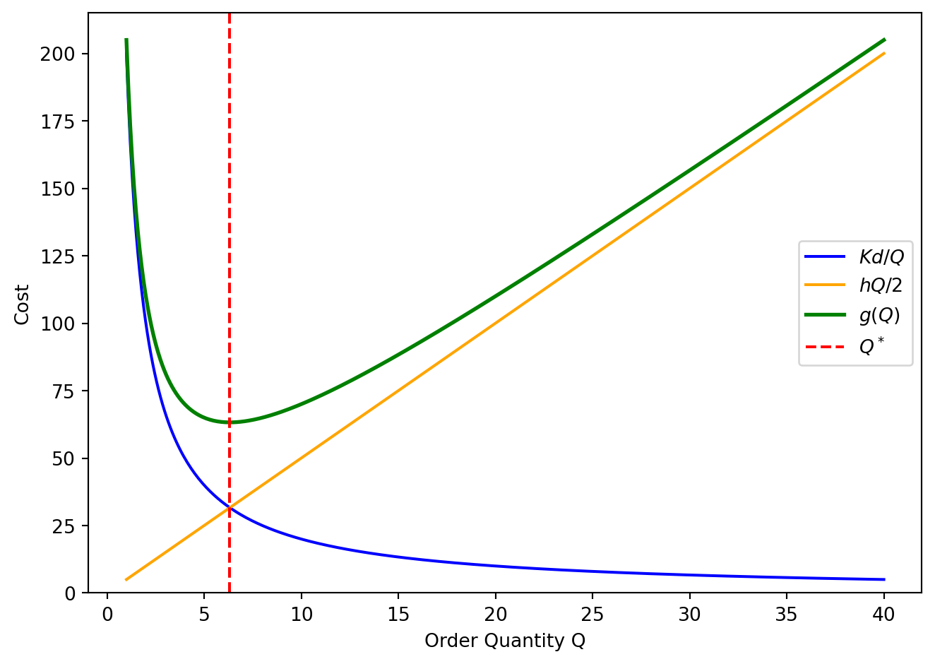
図 14.2 は，購入単価を c = 0 とするときの平均コスト g(Q)，発注コスト \frac{Kd}{Q}，保管コスト \frac{hQ}{2} のグラフである．

import matplotlib.pyplot as plt
import numpy as np

# Parameters
K = 40  # Order cost
h = 10  # Holding cost
d = 5  # Demand rate
Q = np.linspace(1, 40, 400)  # Order quantity from 1 to 40

# Cost calculations
order_cost = K * d / Q
holding_cost = (h * Q) / 2
average_cost = order_cost + holding_cost
optimal_Q = np.sqrt(2 * K * d / h)

# Plotting the costs
# Brand palette, spread over L* = 46 / 58 / 32 so the curves stay apart
# in grayscale and under colour-vision deficiency
plt.plot(Q, order_cost, label=r"$Kd/Q$", color="#137a72")
plt.plot(Q, holding_cost, label=r"$hQ/2$", color="#c17c18")
plt.plot(Q, average_cost, label=r"$g(Q)$", color="#144f78", linewidth=2)
plt.axvline(optimal_Q, color="#b03535", linestyle="--", label=r"$Q^*$")
# The two cost curves cross exactly at Q*
plt.plot(optimal_Q, K * d / optimal_Q, "o", color="#16212d", alpha=0.5, zorder=5)
plt.xlabel("Order Quantity Q")
plt.ylabel("Cost")
plt.ylim(bottom=0)
plt.legend()
plt.tight_layout()
plt.show()

図 14.2: 発注量 Q と平均コスト（K = 40，h = 10，d = 5，c = 0）

図から読み取れるように，Q が増加すると発注コストは減少し，保管コストは増加する．そして平均コストが最小となる点は，この2つの曲線の交点と一致する．すなわち，最適発注量とは発注コストと保管コストを等しくする発注量でもある．実際，両者を等しいとおくと

\frac{Kd}{Q^*} = \frac{hQ^*}{2} \Longrightarrow Q^* = \sqrt{\frac{2Kd}{h}}

となり，定理 14.1 と一致する．

例 14.2 ある電気量販店では，毎月250台のPCが販売されている．発注費用は5000円，保管費用は1台あたり月150円，購入単価は10万円とする．このとき，最適発注量 Q^* は次のように求められる．

Q^* = \sqrt{\frac{2 \cdot 5000 \cdot 250}{150}} \approx 129.10 \text{ 台}

PCの場合は，注文量が整数である必要があるため，g(129) と g(130) を比較する．購入費用の項 cd は Q に依存せず大小関係に影響しないため，以下では省略する．

g(129) = \frac{5000 \cdot 250}{129} + \frac{150 \cdot 129}{2} \approx 19364.92 g(130) = \frac{5000 \cdot 250}{130} + \frac{150 \cdot 130}{2} \approx 19365.38

g(129) < g(130) であるため，最適発注量は Q^* = 129 台となる．

14.8 Excel と Python による計算

14.8.1 Excel

Excel では，SQRT 関数を用いてEOQ公式を計算できる．例 14.2 の場合は，次のようになる．

=SQRT(2 * 5000 * 250 / 150)

14.8.2 Python

Python では，次のようにeoq(K, d, h) 関数を定義し，最適発注量を計算できる．

import numpy as np


def eoq(K, d, h):
    """
    Calculate the Economic Order Quantity (EOQ).

    Parameters:
    K (float): Order cost
    d (float): Demand rate
    h (float): Holding cost

    Returns:
    float: Optimal order quantity Q*
    """
    return np.sqrt(2 * K * d / h)


if __name__ == "__main__":
    K = 5000  # Order cost
    d = 250  # Demand rate (units per month)
    h = 150  # Holding cost (per unit per month)

    Q_star = eoq(K, d, h)
    T_star = Q_star / d
    print(f"Optimal Order Quantity (Q*): {Q_star:.2f}")
    print(f"Optimal Cycle Time (T*): {T_star:.2f}")

Optimal Order Quantity (Q*): 129.10
Optimal Cycle Time (T*): 0.52

14.9 リードタイム*

EOQモデルでは，リードタイムは0と仮定している．リードタイムが L > 0 の場合でも最適発注量 Q^* は変わらず，納品してほしい時点の L 期間前に発注すればよい．変わるのは発注量ではなく，発注のタイミングだけである．

在庫量がある水準 r に達した時点で発注することにし，この r を発注点（reorder point）と呼ぶ．リードタイム L の間に需要は dL 個発生するため，発注点は次のように表される．

r = dL

警告r = dL が使えるのは L < T^* のときだけ

r = dL は，発注してから納品されるまでに，未納品の発注が高々1件しかないことを前提としている．L \geq T^* の場合は，前の発注が届く前に次の発注時点が来るため，発注点は r = dL - \lfloor L / T^* \rfloor Q^* とする必要がある．

例 14.3 例 14.2 において，リードタイムを1週間とし，1ヶ月を4週間とすると，L = 1/4 ヶ月となる．このとき T^* = Q^*/d \approx 0.52 ヶ月であり，L < T^* が成り立つため，r = dL を用いてよい．したがって，発注点は

r = dL = 250 \times \frac{1}{4} = 62.5

となり，PCの在庫量が63台になった時点で発注を行う．

14.10 まとめ

• EOQモデルは，需要率 d が一定，リードタイムが0，欠品を許さない連続観測の在庫モデルである．最適解は，在庫量が0のときに発注し（ZIO），発注量が一定であるという2つの性質をもつ．
• 平均コストは g(Q) = \frac{Kd}{Q} + cd + \frac{hQ}{2} で与えられる．
• g'(Q) = 0 を解くと，EOQ公式 Q^* = \sqrt{2Kd/h} が得られる．g''(Q) > 0 であるため，Q^* は最小値を与える．最適サイクル期間は T^* = Q^*/d である．
• h が増加すると Q^* は減少し，K または d が増加すると Q^* は増加する．購入単価 c は Q^* に影響しない．
• 最適発注量は，発注コストと保管コストが等しくなる発注量でもある．
• *リードタイムが L > 0 の場合も Q^* は変わらず，発注点 r = dL で発注すればよい（ただし L < T^* のとき）．
• 本書の他の章も，EOQモデルの仮定をそれぞれ別の方向に緩めたものと見ることができる．需要が確率的な場合は チャプター 15 と チャプター 17 で，需要が期ごとに変化する場合は チャプター 16 で扱う．

14.11 用語集

English	Japanese
Economic Order Quantity (EOQ)	経済的発注量
Deterministic	決定論的
Constant	一定
Demand Rate	需要率
Fixed Cost	固定費用
Cycle	サイクル
Inventory Level	在庫量
Order Quantity	発注量
EOQ Formula	EOQ公式
Lead Time	リードタイム
Reorder Point	発注点

14.12 文献案内

オペレーションズ・リサーチに関する教科書の多くは，EOQモデルを取り扱っている．モデルの分類から，「deterministic continuous-review inventory models」などの章で説明されていることが多い．リードタイムを考慮したEOQモデルについては，Snyder と Shen (2019年) で説明されている．

本章の仮定をさらに緩めると，EOQモデルは次のように拡張される．いずれも本書では扱わないが，文献を挙げておく．

• バックオーダーを考慮したEOQモデル（欠品を許す）：Snyder と Shen (2019年)，Camm ほか (2022年)，Hillier と Lieberman (2025年)
• 数量割引（quantity discount）を考慮したEOQモデル（購入単価 c が発注量に依存する）：Snyder と Shen (2019年)，Camm ほか (2022年)
  • 総量割引（all-units discount）
  • 増分割引（incremental discount）

14.13 練習問題

練習 14.1 需要率を d，発注費用を K，保管費用を h，購入単価を c とする．

1. EOQモデルにおける平均コスト g(Q) を発注量 Q の関数として導出せよ．
2. g(Q) を最小化する発注量 Q^* を導出せよ．また，なぜ Q^* が最小値を与えるのか説明せよ．

解答 14.1. 1. 1サイクルあたりのコストは，発注費用 K，購入費用 cQ，保管費用 \frac{hQ^2}{2d} の和である．保管費用は，平均在庫量 \frac{Q}{2} がサイクル期間 T = \frac{Q}{d} にわたって保管されることから得られる．これをサイクル期間 T で割ると，

g(Q) = \frac{d}{Q} \left( K + cQ + \frac{hQ^2}{2d} \right) = \frac{Kd}{Q} + cd + \frac{hQ}{2}

となる．

2. g'(Q) = 0 とすると，

g'(Q) = -\frac{Kd}{Q^2} + \frac{h}{2} = 0 \Longrightarrow Q^* = \sqrt{\frac{2Kd}{h}}

を得る．Q > 0 において g''(Q) = \frac{2Kd}{Q^3} > 0 であり，g(Q) は下に凸である．したがって，g'(Q^*) = 0 を満たす Q^* は最小値を与える．

練習 14.2 (EOQ for Vaccines) ある病院では，毎月300本のワクチンを使用している．ワクチンの製造業者に発注するたびに，固定費用として100ドルがかかる．ワクチン1本あたりの保管費用は，年間3ドルである．EOQモデルを用いて，次の問いに答えよ．

1. 最適な発注量 Q^* を求めよ．
2. 固定費用が減少した場合，最適発注量はどのように変化するか説明せよ．

練習 14.3 EOQモデルに基づき，次の各条件の変化が最適発注量 Q^* にどのような影響を与えるかを説明せよ．

1. 発注費用が2倍になった場合．
2. 保管費用が0.25倍になった場合．
3. 需要率が4倍になった場合

練習 14.4 (EOQ for Steel) ある工場は，鋼材を毎日16トン消費し，年間250日稼働している．鋼材の購入単価は1トンあたり1100ドル，1回の発注にかかる固定費は5500ドル，保管費は鋼材1トンあたり年間275ドルである．EOQモデルを用いて，次の問いに答えよ．

1. 最適な発注量を求めよ．
2. 最適なサイクル期間を求めよ．
3. 年間の平均費用を求めよ．

練習 14.5 (EOQ for Smartphones) ある家電量販店では，あるスマートフォンを毎週50台販売している．店舗はスマートフォンを1台あたりメーカーに10万円で購入している．毎回の発注には発注処理や配送などで5000円の固定費がかかる．また，スマートフォン1台あたりの保管費用は1週間で100円である．EOQモデルを用いて，次の問いに答えよ．

1. 最適な発注量を求めよ．
2. 最適なサイクル期間を求めよ．

解答 14.2. 需要率は d = 50 で，発注費用は K = 5000，保管費用は h = 100 である．

経済的発注量 Q^* は Q^* = \sqrt{\frac{2Kd}{h}} = \sqrt{\frac{2 \cdot 5000 \cdot 50}{100}} \approx 70.71 \text{ 台} となる．スマートフォンの場合は，注文量が整数である必要があるため，g(70) と g(71) を比較して最適発注量を決定する．購入費用の項 cd は Q に依存せず大小関係に影響しないため，以下では省略する．

g(70) = \frac{5000 \cdot 50}{70} + 100 \cdot 70 / 2 \approx 7071.43 g(71) = \frac{5000 \cdot 50}{71} + 100 \cdot 71 / 2 \approx 7071.13 g(71) < g(70) であるため，最適発注量は Q^* = 71 台となる．

サイクル期間 T^* は T^* = \frac{Q^*}{d} = \frac{71}{50} = 1.42 \text{ 週間} となる．

import numpy as np

K = 5000  # Order cost
d = 50  # Demand rate (units per week)
h = 100  # Holding cost (per unit per week)
Q_star = np.sqrt(2 * K * d / h)


# Since order quantity must be an integer, compare g(70) and g(71)
def g(Q):
    return (K * d / Q) + (h * Q / 2)


g_70 = g(70)
g_71 = g(71)
optimal_Q = 70 if g_70 < g_71 else 71
T_star = optimal_Q / d
print(f"Optimal Order Quantity (Q*): {optimal_Q} units")
print(f"Optimal Cycle Time (T*): {T_star:.2f} weeks")

Optimal Order Quantity (Q*): 71 units
Optimal Cycle Time (T*): 1.42 weeks

Camm, Jeffrey, James Cochran, Michael Fry, ほか. 2022年. An introduction to management science: Quantitative approaches to decision making. 16番目 版. South-Western College Publishing.

Harris, Ford W. 1990年. 「How many parts to make at once」. Oper. Res. 38 (6): 947–50.

Hillier, Frederick, と Gerald Lieberman. 2025年. ISE introduction to operations research. 11番目 版. McGraw-Hill Education.

Snyder, Lawrence V, と Zuo-Jun Max Shen. 2019年. Fundamentals of supply chain theory. 2番目 版. John Wiley & Sons.