動的計画法による最短路問題とナップサック問題の解法を理解する.
動的計画法の基本的な考え方を理解する.
*ベルマン方程式の意味を理解する.
動的計画法 (dynamic programming, DP)は Richard E. Bellman によって提案された,多段階決定過程 (multi-stage decision process)に対する最適化手法である.
動的計画法を algorithmic paradigm の一つとして扱う場合もあるが,本書では最適化手法として説明する.
多段階決定過程は,複数の段階にわたって行われる一連の意思決定を行う問題である.各段階において,意思決定者は現在の状態 を観測し,意思決定を行う.その意思決定は,将来の状態に影響を与える.目的として,状態に関するある目的関数を最小化(または最大化)することである.動的計画法は,多段階決定過程における最適方策 (optimal policy)を求めるための一般的な手法である.
経営工学,制御工学、経済学,生物学などの分野において,多数の応用例が知られている.例えば,
などである.さらに,現在では,強化学習の基礎理論としても重要な役割を果たしている.
ここでは,最短路問題 (shortest path problem)とナップサック問題 (knapsack problem)を例に,動的計画法の基本的な考え方を説明する.
I spent the Fall quarter (of 1950) at RAND. My first task was to find a name for multistage decision processes. An interesting question is, “Where did the name, dynamic programming, come from?” The 1950s were not good years for mathematical research. We had a very interesting gentleman in Washington named Wilson. He was Secretary of Defense, and he actually had a pathological fear and hatred of the word “research”. I’m not using the term lightly; I’m using it precisely. His face would suffuse, he would turn red, and he would get violent if people used the term research in his presence. You can imagine how he felt, then, about the term mathematical. The RAND Corporation was employed by the Air Force, and the Air Force had Wilson as its boss, essentially. Hence, I felt I had to do something to shield Wilson and the Air Force from the fact that I was really doing mathematics inside the RAND Corporation. What title, what name, could I choose? In the first place I was interested in planning, in decision making, in thinking. But planning, is not a good word for various reasons. I decided therefore to use the word “programming”. I wanted to get across the idea that this was dynamic, this was multistage, this was time-varying. I thought, let’s kill two birds with one stone. Let’s take a word that has an absolutely precise meaning, namely dynamic, in the classical physical sense. It also has a very interesting property as an adjective, and that is it’s impossible to use the word dynamic in a pejorative sense. Try thinking of some combination that will possibly give it a pejorative meaning. It’s impossible. Thus, I thought dynamic programming was a good name. It was something not even a Congressman could object to. So I used it as an umbrella for my activities.
— Richard Bellman, Eye of the Hurricane: An Autobiography (1984, page 159)
最短路問題
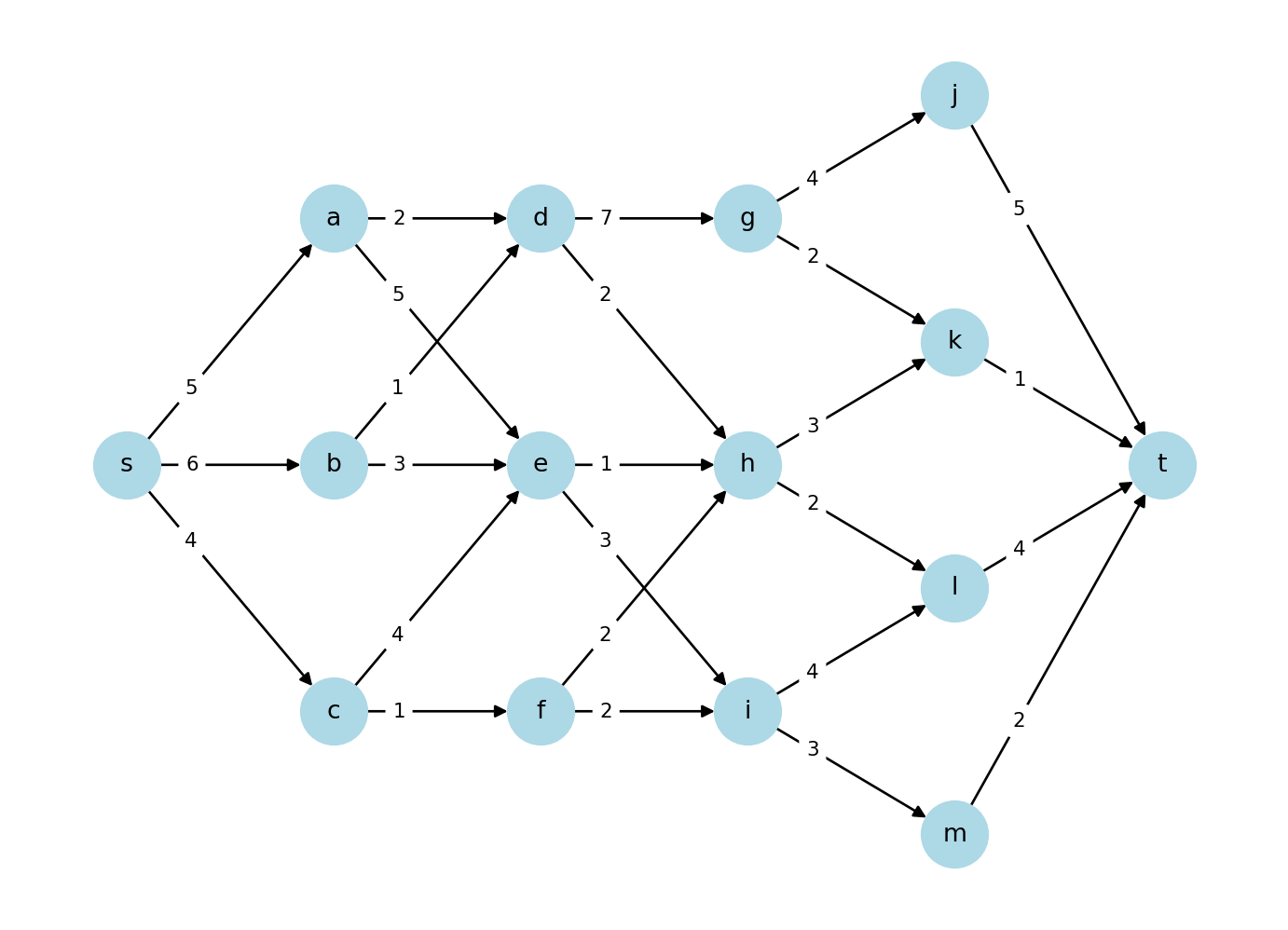
多段階の有向グラフ \(G = (V, E)\) における最短路問題を考える. 各辺 \((v, u) \in E\) に非負の重み \(w(v, u)\) が与えられているとする.始点 \(s \in V\) から終点 \(t \in V\) への最短路を求める問題である.\(s\) と \(t\) 以外の頂点を段階 \(D = \{ 1, 2, \ldots, n \}\) に分けることができるとする.結果として,\(n\) 回の意思決定を行い,最適解は \((s, v_1, v_2, \ldots, v_n, t)\) の形になる.
\(P^* = (s, v_1, v_2, \ldots, v_n, t)\) は最短路であれば,任意の \(1 \leq k \leq n\) に対して,パス \((v_k, v_{k+1}, \ldots, v_n, t)\) も \(v_k\) から \(t\) への最短路である.これは,もし \((v_k, v_{k+1}, \ldots, v_n, t)\) が最短路でないとすると,より短いパスが存在し,\(P^*\) も最短路でなくなるためである.この性質は最適性の原理 (Principle of Optimality)と呼ばれる.Bellman は次のように述べている.
最適性の原理 (Principle of Optimality):最適な方策は、初期状態と初期決定がどんなものであれ、その結果得られる次の状態に関して、以降の決定が必ず最適方策になっているという性質をもつ.
– Richard Bellman, 1957
点 \(v\) から点 \(t\) までの最短路の長さ(またはコスト)を \(d(v)\) と定義する.最適性の原理により,点 \(v \in V \setminus \{ t \}\) に対して,
\[
d(v) = \min_{u \in \mathcal{S}(v)} \{ w(v, u) + d(u) \}
\]
が成り立つ.ここで,\(\mathcal{S}(v) = \{ u \mid (v, u) \in E \}\) とする.
例 13.1 \(d(a) = 8\) ,\(d(b) = 7\) ,\(d(c) = 7\) が与えられたとき,\(d(s)\) を計算せよ.
コード
import networkx as nximport matplotlib.pyplot as plt= nx.DiGraph()= ["s" , "a" , 5 ),"s" , "b" , 6 ),"s" , "c" , 4 ),"a" , "d" , 2 ),"a" , "e" , 5 ),"b" , "d" , 1 ),"b" , "e" , 3 ),"c" , "e" , 4 ),"c" , "f" , 1 ),"d" , "g" , 7 ),"d" , "h" , 2 ),"e" , "h" , 1 ),"e" , "i" , 3 ),"f" , "h" , 2 ),"f" , "i" , 2 ),"g" , "j" , 4 ),"g" , "k" , 2 ),"h" , "k" , 3 ),"h" , "l" , 2 ),"i" , "l" , 4 ),"i" , "m" , 3 ),"j" , "t" , 5 ),"k" , "t" , 1 ),"l" , "t" , 4 ),"m" , "t" , 2 ),for layer, nodes in enumerate (nx.topological_generations(G)):for node in nodes:"layer" ] = layer= {"s" : (0 , 0 ),"a" : (1 , 1 ),"b" : (1 , 0 ),"c" : (1 , - 1 ),"d" : (2 , 1 ),"e" : (2 , 0 ),"f" : (2 , - 1 ),"g" : (3 , 1 ),"h" : (3 , 0 ),"i" : (3 , - 1 ),"j" : (4 , 1.5 ),"k" : (4 , 0.5 ),"l" : (4 , - 0.5 ),"m" : (4 , - 1.5 ),"t" : (5 , 0 ),= True ,= 800 ,= "white" ,= 12 ,= "black" ,= nx.get_edge_attributes(G, "weight" )= edge_labels, label_pos= 0.3 , font_size= 10 , rotate= False
コード
# find shortest path from s to t = "s" = "t" = nx.shortest_path(G, source= source, target= target, weight= "weight" )= nx.shortest_path_length(= source, target= target, weight= "weight" # shortest_path, shortest_path_length
\[\begin{align*}
d(s) &= \min \{ w(s, a) + d(a), w(s, b) + d(b), w(s, c) + d(c) \} \\
&= \min \{ 5 + 8, 6 + 7, 4 + 7 \} \\
&= \min \{ 13, 13, 11 \} \\
&= 11
\end{align*}\]
さらに,\(w(s, c) + d(c)\) が最小値を与えるため,最短路は \((s, c, ..., t)\) にあることがわかる.
例 13.1 の考え方を一般化し,動的計画法による最短路問題の解法を以下のアルゴリズムに示す.
Algorithm 13.1
Input : 有向グラフ \(G = (V, E)\) ,重み関数 \(w: E \to \mathbb{R}_{\geq 0}\) ,始点 \(s \in V\) ,終点 \(t \in V\) Output : \(s\) から \(t\) への最短路の長さ \(d(s)\)
\(d(t) \leftarrow 0\) \(d(v) \leftarrow \infty\) for all \(v \in V \setminus \{ t \}\) \(k \leftarrow n-1\) while \(k \geq 0\) do
for each \(v \in D_k\) do
\(d(v) \leftarrow \min_{u \in \mathcal{P}(v)} \{ w(v, u) + d(u) \}\)
\(k \leftarrow k - 1\)
return \(d(s)\)
def dp_shortest_path(G):# Initialize distances = {v: float ("inf" ) for v in G.nodes()}"t" ] = 0 # Distance to target is 0 # Get layers in topological order = list (nx.topological_generations(G))# Process layers in reverse order for layer in reversed (layers[:- 1 ]): # Exclude the last layer (target) for v in layer:= min ("weight" ] + d[u] for u in G.successors(v)),return d["s" ]if __name__ == "__main__" := dp_shortest_path(G)print (shortest_path_length_dp)
まず,\(d(t) = 0\) とし,第 4 段の点 \(j\) ,\(k\) ,\(l\) ,\(m\) について,\(d(j)\) ,\(d(k)\) ,\(d(l)\) ,\(d(m)\) を計算する.
\[\begin{align*}
d(j) &= \min \{ w(j, t) + d(t) \} = \min \{ 5 + 0 \} = 5 \\
d(k) &= \min \{ w(k, t) + d(t) \} = \min \{ 1 + 0 \} = 1 \\
d(l) &= \min \{ w(l, t) + d(t) \} = \min \{ 4 + 0 \} = 4 \\
d(m) &= \min \{ w(m, t) + d(t) \} = \min \{ 2 + 0 \} = 2 \\
\end{align*}\]
次に,第 3 段の点 \(g\) ,\(h\) ,\(i\) について,\(d(g)\) ,\(d(h)\) ,\(d(i)\) を計算する.
\[\begin{align*}
d(g) &= \min \{ w(g, j) + d(j), w(g, k) + d(k) \} \\
&= \min \{ 4 + 5, 2 + 1 \} = 3 \\
d(h) &= \min \{ w(h, k) + d(k), w(h, l) + d(l) \} \\
&= \min \{ 3 + 1, 2 + 4 \} = 4 \\
d(i) &= \min \{ w(i, l) + d(l), w(i, m) + d(m) \} \\
&= \min \{ 4 + 4, 3 + 2 \} = 5 \\
\end{align*}\]
第 2 段の点 \(d\) ,\(e\) ,\(f\) について,\(d(d)\) ,\(d(e)\) ,\(d(f)\) を計算する.
\[\begin{align*}
d(d) &= \min \{ w(d, g) + d(g), w(d, h) + d(h) \} \\
&= \min \{ 7 + 3, 2 + 4 \} = 6 \\
d(e) &= \min \{ w(e, h) + d(h), w(e, i) + d(i) \} \\
&= \min \{ 1 + 4, 3 + 5 \} = 5 \\
d(f) &= \min \{ w(f, h) + d(h), w(f, i) + d(i) \} \\
&= \min \{ 2 + 4, 2 + 5 \} = 6 \\
\end{align*}\]
第 1 段の点 \(a\) ,\(b\) ,\(c\) について,\(d(a)\) ,\(d(b)\) ,\(d(c)\) を計算する.
\[\begin{align*}
d(a) &= \min \{ w(a, d) + d(d), w(a, e) + d(e) \} \\
&= \min \{ 2 + 6, 5 + 5 \} = 8 \\
d(b) &= \min \{ w(b, d) + d(d), w(b, e) + d(e) \} \\
&= \min \{ 1 + 6, 3 + 5 \} = 7 \\
d(c) &= \min \{ w(c, e) + d(e), w(c, f) + d(f) \} \\
&= \min \{ 4 + 5, 1 + 6 \} = 7 \\
\end{align*}\]
最後に,始点 \(s\) について,\(d(s)\) を計算する.
\[\begin{align*}
d(s) &= \min \{ w(s, a) + d(a), w(s, b) + d(b), w(s, c) + d(c) \} \\
&= \min \{ 5 + 8, 6 + 7, 4 + 7 \} \\
&= \min \{ 13, 13, 11 \} \\
&= 11
\end{align*}\]
最短路 \(P^*\) は,\(d(s)\) の計算過程を逆にたどることで求めることができる.点 \(v\) に対して,次の点 \(u\) を
\[
u = \arg \min_{u' \in \mathcal{P}(v)} \{ w(v, u') + d(u') \}
\]
と定義する.ここで,\(\mathcal{P}(v) = \{ u \mid (v, u) \in E \}\) である.始点 \(s\) から始めて,次の点を順にたどることで,最短路 \(P^*\) を構築できる.
例えば,\(w(s, a) + d(a) = 13\) ,\(w(s, b) + d(b) = 13\) ,\(w(s, c) + d(c) = 11\) であるため,\(w(s, c) + d(c)\) が最小値を与え,次は \(c\) である.同様にたどると,最短路は \((s, c, f, i, m, t)\) となる.
例 13.2 \(v\) から点 \(t\) までの最長路の長さ \(d(v)\) は, \[
d(v) = \max_{u \in \mathcal{P}(v)} \{ w(v, u) + d(u) \}
\] と与えられる.
0/1 ナップサック問題
0/1 ナップサック問題は,有限個の品物からなる集合 \(I = \{ 1, 2, \ldots, n \}\) と,ナップサックの容量 \(W\) が与えられたとき,以下の最適化問題を解くことである.
\[\begin{align*}
\text{maximize} \quad & \sum_{i \in I} v_i x_i \\
\text{subject to} \quad & \sum_{i \in I} w_i x_i \leq W \\
& x_i \in \{ 0, 1 \} \quad \forall i \in I
\end{align*}\]
ここで,\(v_i\) は品物 \(i\) の価値,\(w_i\) は品物 \(i\) の重量,\(x_i\) は品物 \(i\) をナップサックに入れるかどうかを示す 0/1 変数である.目的は,ナップサックの容量を超えないように品物を選び,その価値の総和を最大化することである.
下では,0/1 ナップサック問題の例題を示す.
例 13.3 (0/1 ナップサック問題の例) \(W = 15\) ,品物の集合 \(I = \{ 1, 2, 3, 4 \}\) とし,各品物の重量 \(w_i\) と価値 \(v_i\) を以下の表に示す.\(\mathbf{x} = (x_1, x_2, x_3, x_4)\) とすると,最適解を求めよ.
最適解は \(\mathbf{x^*} = (1, 1, 0, 1)\) であり,価値の総和は 8 である.
動的計画法を用いて,0/1 ナップサック問題を解く方法を説明するため,0/1 ナップサック問題を,品物 \(1, 2, \ldots, n\) を取るか取らないかを順に決定していく多段階決定過程として定式化する.すなわち,段階 \(i\) において,品物 \(i\) を取るか取らないかを決定する.
この問題において,\(\mathbf{x^*} = (x_1, x_2, \ldots, x_n)\) は最適解であれば,\((x_i, x_{i+1}, \ldots, x_n)\) は,利用可能な容量が \(W - \sum_{j=1}^{i-1} w_j x_j\) のときの品物 \(i, i+1, \ldots, n\) に対する最適解である.これは,もし \((x_i, x_{i+1}, \ldots, x_n)\) が最適解でないとすると,より価値の高い解が存在し,\(\mathbf{x^*}\) も最適解でなくなるためである.
\(v_i(w)\) を,品物 \(i, i+1, \ldots, n\) から選んで,利用可能な容量が \(w\) のときの最大価値と定義する.すなわち,\(v_i(w)\) は,以下の最適化問題の最適値を与える.
\[\begin{align*}
\text{maximize} \quad & \sum_{j = i}^{n} v_j x_j \\
\text{subject to} \quad & \sum_{j = i}^{n} w_j x_j \leq w \\
& x_j \in \{ 0, 1 \} \quad \forall j = i, i+1, \ldots, n
\end{align*}\]
明らかに,\(v_1(W)\) は原問題の最適値である.
再帰方程式を導出するために,品物 \(i\) の重量 \(w_i\) と利用可能な容量 \(w\) を比較する.\(w_i > w\) の場合,品物 \(i\) の重量 \(w_i\) が利用可能な容量 \(w\) を超え,品物 \(i\) は取れないため, \[
v_i(w) = v_{i+1}(w)
\] となる.
\(w_i \leq w\) の場合,品物 \(i\) を取らない場合と取る場合のうち,価値の高い方を選ぶ.品物 \(i\) を取らない場合は,利用可能な容量が \(w\) のままで,価値は \(v_{i+1}(w)\) である.品物 \(i\) を取る場合は,利用可能な容量が \(w - w_i\) となり,価値は \(v_{i+1}(w - w_i) + v_i\) である.したがって, \[
v_i(w) = \max \{ v_{i+1}(w), v_{i+1}(w - w_i) + v_i \}
\] となる.
以上の説明により,\(v_i(w)\) は以下の再帰方程式で与えられる.
\[
v_i(w) =
\begin{cases}
v_{i+1}(w) & \text{if } w_i > w \\
\max \{ v_{i+1}(w), v_{i+1}(w - w_i) + v_i \} & \text{if } w_i \leq w
\end{cases}
\]
また,\(n+1\) 段階目では品物が存在しないため,すべての容量 \(w\) に対して \(v_{n+1}(w) = 0\) となる.
\(v_1(W)\) を計算するために,すべての \(w = 0, 1, \ldots, W\) に対して,\(v_n(w), \ldots, v_1(w)\) を順に計算する.この方法を用いた 0/1 ナップサック問題の動的計画法による解法を以下のアルゴリズムに示す.
Algorithm 13.2
Input : 品物の集合 \(I = \{ 1, 2, \ldots, n \}\) ,品物 \(i\) の重量 \(w_i\) ,品物 \(i\) の価値 \(v_i\) ,ナップサックの容量 \(W\) Output : 最適値 \(v_1(W)\)
for all \(w = 0, 1, \ldots, W\) do
\(v_{n+1}(w) \leftarrow 0\)
for \(i = n, n-1, \ldots, 1\) do
for all \(w = 0, 1, \ldots, W\) do
if \(w_i > w\) then
\(v_i(w) \leftarrow v_{i+1}(w)\)
else
\(v_i(w) \leftarrow \max \{ v_{i+1}(w), v_{i+1}(w - w_i) + v_i \}\)
return \(v_1(W)\)
def dp_knapsack(weights, values, W):= len (weights)# Initialize value table = [[0 for _ in range (W + 1 )] for _ in range (n + 2 )]# Fill the table in reverse order for i in range (n, 0 , - 1 ):for w in range (W + 1 ):if weights[i - 1 ] > w:= v[i + 1 ][w]else := max (v[i + 1 ][w], v[i + 1 ][w - weights[i - 1 ]] + values[i - 1 ])return v[1 ][W]if __name__ == "__main__" := [12 , 2 , 1 , 1 ]= [4 , 2 , 1 , 2 ]= 15 = dp_knapsack(weights, values, W)print (optimal_value) # Output: 8
例 13.3 の例題に対して,容量 \(W = 2\) のときの計算過程を以下に示す.
すべての \(w = 0, 1, 2\) に対して \(v_5(w) = 0\) とする.品物 \(i = 4\) の重量と価値はそれぞれ \(w_4 = 1\) ,\(v_4 = 2\) であり,\(w = 0, 1, 2\) に対して \(v_4(w)\) を計算し,
\[\begin{align*}
v_4(0) &= 0 \\
v_4(1) &= \max \{ v_5(1), v_5(0) + 2 \} = \max \{ 0, 0 + 2 \} = 2 \\
v_4(2) &= \max \{ v_5(2), v_5(1) + 2 \} = \max \{ 0, 0 + 2 \} = 2 \\
\end{align*}\]
が得られる.次に \(i = 3\) について,次の結果が得られる.
\[\begin{align*}
v_3(0) &= 0 \\
v_3(1) &= \max \{ v_4(1), v_4(0) + 1 \} = \max \{ 2, 0 + 1 \} = 2 \\
v_3(2) &= \max \{ v_4(2), v_4(1) + 1 \} = \max \{ 2, 2 + 1 \} = 3 \\
\end{align*}\]
次に \(i = 2\) について,次の結果が得られる. \[\begin{align*}
v_2(0) &= 0 \\
v_2(1) &= v_3(1) = 2 \\
v_2(2) &= \max \{ v_3(2), v_3(0) + 2 \} = \max \{ 3, 0 + 2 \} = 3 \\
\end{align*}\]
最後に \(i = 1\) について,\(w_1 = 12 > 2\) より,次の結果が得られる. \[
v_1(2) = v_2(2) = 3
\] が得られる.したがって,最適値は \(v_1(2) = 3\) である.最適解は,計算過程を逆にたどることで求めることができる.下に示すように,最適解は \(\mathbf{x^*} = (0, 0, 1, 1)\) である.
\(v_1(2) = v_2(2)\) より,品物 1 は取らない.\(x_1^* = 0\) .\(v_2(2) = v_3(2)\) より,品物 2 は取らない.\(x_2^* = 0\) .\(v_3(2) = v_4(1) + 1\) より,品物 3 は取る.\(x_3^* = 1\) .利用可能な容量は \(2 - 1 = 1\) となる.\(v_4(1) = v_5(0) + 2\) より,品物 4 は取る.\(x_4^* = 1\) .
ベルマン方程式(確定的場合)*
動的計画法における最適性の原理は,ベルマン方程式 (Bellman equation)として知られる再帰方程式により表現される.状態 \(s\) におけるの価値関数 \(v(s)\) は,以下のように定義される.
\[
v(s) = \max_{a \in A(s)} \{ r(s, a) + \gamma v(s') \}
\]
ここで,\(A(s)\) は状態 \(s\) における可能な行動の集合,\(r(s, a)\) は状態 \(s\) で行動 \(a\) を取ったときの報酬,\(\gamma\) は割引率,\(s'\) は行動 \(a\) を取った後の次の状態である.
\(s\) 現在の頂点
現在の品物と利用可能な容量
\(a\) 次に移動する頂点
品物を取るか取らないか
\(A(s)\) 現在の頂点から到達可能な頂点の集合
現在の品物を取るか取らないかの選択肢
\(R(s, a)\) 負の辺の重み
品物の価値
\(s'\) 次の頂点
次の品物と新しい利用可能な容量
演習問題
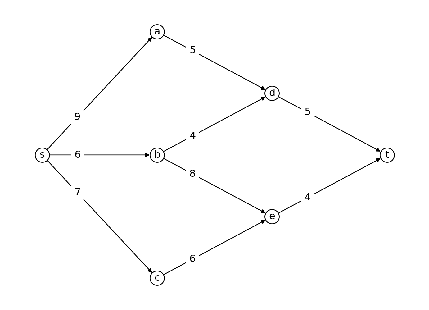
練習 13.1 \(s\) から終点 \(t\) への最短路を求めよ.
コード
import networkx as nximport matplotlib.pyplot as plt= nx.DiGraph()= ["s" , "a" , 9 ),"s" , "b" , 6 ),"s" , "c" , 7 ),"a" , "d" , 5 ),"b" , "d" , 4 ),"b" , "e" , 8 ),"c" , "e" , 6 ),"d" , "t" , 5 ),"e" , "t" , 4 ),= {"s" : (0 , 0 ),"a" : (1 , 1 ),"b" : (1 , 0 ),"c" : (1 , - 1 ),"d" : (2 , 0.5 ),"e" : (2 , - 0.5 ),"t" : (3 , 0 ),= True ,= 300 ,= "white" ,= 12 ,= "black" ,= nx.get_edge_attributes(G, "weight" )= edge_labels, label_pos= 0.3 , font_size= 12 , rotate= False # # find shortest path from s to t # source = "s" # target = "t" # shortest_path = nx.shortest_path(G, source=source, target=target, weight="weight") # shortest_path_length = nx.shortest_path_length( # G, source=source, target=target, weight="weight" # ) # shortest_path, shortest_path_length # print(shortest_path, shortest_path_length)
解答 13.1 . \(v\) から点 \(t\) までの最短路の長さを \(d(v)\) と表し,以下のように計算する. \[
d(v) = \min_{u \in \mathcal{S}(v)} \{ w(v, u) + d(u) \}
\]
次に,段階ごとに \(d(v)\) を計算する.ここで,\(t, d, e, a, b, c, s\) の順に計算する.
\[\begin{align*}
d(t) &= 0 \\
d(d) &= \min \{ w(d, t) + d(t) \} = \min \{ 5 + 0 \} = 5 \\
d(e) &= \min \{ w(e, t) + d(t) \} = \min \{ 4 + 0 \} = 4 \\
d(a) &= \min \{ w(a, d) + d(d) \} = \min \{ 5 + 5 \} = 10 \\
d(b) &= \min \{ w(b, d) + d(d), w(b, e) + d(e) \} \\
&= \min \{ 4 + 5, 8 + 4 \} = \min \{ 9, 12 \} = 9 \\
d(c) &= \min \{ w(c, e) + d(e) \} = \min \{ 6 + 4 \} = 10 \\
d(s) &= \min \{ w(s, a) + d(a), w(s, b) + d(b), w(s, c) + d(c) \} \\
&= \min \{ 9 + 10, 6 + 9, 7 + 10 \} \\
&= \min \{ 19, 15, 17 \} \\
&= 15
\end{align*}\]
したがって,\(s\) から \(t\) への最短路の長さは 15 である.最短路は \(d(s)\) の計算過程を逆にたどることで求めることができ,\(P^* = (s, b, d, t)\) である.
練習 13.2 \(W = 3\) ,品物の集合 \(I = \{ 1, 2, 3, 4 \}\) とし,各品物の重量 \(w_i\) と価値 \(v_i\) を以下の表に示す.
ナップサックの容量 \(W = 3\) のときの最適値と最適解を求めよ.