8  Shortest Path Problem

8.1 Learning Objectives

  • Understand the shortest path problem.
  • Understand Dijkstra’s algorithm and find the shortest path length from the start vertex to each vertex.

8.2 Shortest Path

Consider a directed graph G = (V, E) in which each edge (v, u) \in E has a nonnegative weight w(v, u). In this chapter, the length of a path is the sum of the weights of its edges, not the number of its edges as in Chapter 6. A shortest path from a vertex s \in V to a vertex t \in V is a path from s to t with the smallest length. The shortest path problem is the problem of finding a shortest path from s to t.

Example 8.1 Figure 8.1 shows an example of the shortest path problem.

Code
import math

import matplotlib.pyplot as plt
import networkx as nx

# Computer Modern fonts, as in LaTeX. The last setting avoids a warning about cmr10.
latex_style = {
    "font.family": "cmr10",
    "mathtext.fontset": "cm",
    "axes.formatter.use_mathtext": True,
}


def draw_graph(G, pos, width, height):
    """Draw the directed graph G with the vertices at the positions pos.

    A vertex "v1" is labeled $v_1$. An edge is drawn as an arrow, and its
    weight as a number beside the edge.
    """
    labels = {v: rf"$v_{v[1:]}$" if v.startswith("v") else rf"${v}$" for v in G}
    with plt.rc_context(latex_style):
        fig, ax = plt.subplots(figsize=(width, height))
        nx.draw_networkx(
            G,
            pos,
            labels=labels,
            node_color="white",
            edgecolors="black",
            linewidths=1.0,
            node_size=450,
            font_size=12,
            font_family="cmr10",
            width=1.0,
            arrowstyle="-|>",
            arrowsize=12,
            ax=ax,
        )
        # Each weight is placed beside its edge, on the side away from the center of the graph
        weights = nx.get_edge_attributes(G, "weight")
        cx = sum(x for x, y in pos.values()) / len(pos)
        cy = sum(y for x, y in pos.values()) / len(pos)
        for (v, u), w in weights.items():
            (x1, y1), (x2, y2) = pos[v], pos[u]
            mx, my = (x1 + x2) / 2, (y1 + y2) / 2  # midpoint of the edge
            length = math.hypot(x2 - x1, y2 - y1)
            px, py = (y1 - y2) / length, (x2 - x1) / length  # unit vector perpendicular to the edge
            if px * (mx - cx) + py * (my - cy) < 0:
                px, py = -px, -py
            ax.annotate(
                str(w), (mx, my), xytext=(7 * px, 7 * py), textcoords="offset points",
                ha="center", va="center", fontsize=10,
            )
        ax.set_aspect("equal")
        ax.margins(0.12)
        ax.axis("off")
        plt.show()


G = nx.DiGraph()
G.add_weighted_edges_from([
    ("s", "v1", 2), ("s", "v2", 1), ("v1", "v2", 3), ("v1", "v3", 3),
    ("v2", "v4", 1), ("v3", "t", 2), ("v4", "v3", 2), ("v4", "t", 5),
])
pos = {
    "s": (0, 1), "v1": (1.3, 2), "v2": (1.3, 0),
    "v3": (2.6, 2), "v4": (2.6, 0), "t": (3.9, 1),
}
draw_graph(G, pos, 4.5, 2.4)
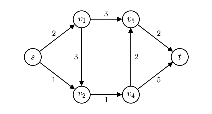
A directed graph with six vertices drawn as circles labeled s, v1, v2, v3, v4, and t. Vertex s is at the left, v1 and v3 are in the top row, v2 and v4 are in the bottom row, and t is at the right. The edges and their weights are s to v1 with weight 2, s to v2 with weight 1, v1 to v2 with weight 3, v1 to v3 with weight 3, v2 to v4 with weight 1, v3 to t with weight 2, v4 to v3 with weight 2, and v4 to t with weight 5.
Figure 8.1: An example of the shortest path problem. The number on each edge is its weight.

8.3 Dijkstra’s Algorithm

Algorithm 1 shows Dijkstra’s algorithm. Here, d(v) is the length of the shortest path from s to v found so far, W is the set of vertices whose shortest path lengths have been fixed, and \mathcal{S}(v) is the set of successors of v (Chapter 6).

\begin{algorithm} \caption{Dijkstra's Algorithm} \begin{algorithmic} \Require directed graph $G = (V, E)$, weight function $w: E \to \mathbb{R}_{\geq 0}$, start vertex $s \in V$ \Ensure shortest path length $d(v)$ from $s$ to each vertex $v \in V$ \State $W \gets \emptyset$ \ForAll{$v \in V$} \State $d(v) \gets \infty$ \EndFor \State $d(s) \gets 0$ \While{$W \neq V$} \State $v \gets \arg \min_{u \in V \setminus W} d(u)$ \State $W \gets W \cup \{v\}$ \ForAll{$u \in \mathcal{S}(v) \setminus W$} \State $d(u) \gets \min(d(u), d(v) + w(v, u))$ \EndFor \EndWhile \State \textbf{return} $d$ \end{algorithmic} \end{algorithm}

Example 8.2 (Dijkstra’s algorithm) Consider again the directed graph in Figure 8.1. We apply Algorithm 1 with start vertex s.

Table 8.1 shows d(v) after each iteration of the while loop, together with the vertex added to W in the iteration. A value in bold is fixed, that is, its vertex is in W.

Table 8.1: d(v) in Dijkstra’s algorithm from s. The first row shows d(v) before the while loop.
Iteration Added to W d(s) d(v_1) d(v_2) d(v_3) d(v_4) d(t)
– – 0 \infty \infty \infty \infty \infty
1 s 0 2 1 \infty \infty \infty
2 v_2 0 2 1 \infty 2 \infty
3 v_1 0 2 1 5 2 \infty
4 v_4 0 2 1 4 2 7
5 v_3 0 2 1 4 2 6
6 t 0 2 1 4 2 6

In iteration 1, s is added to W, and d(v_1) and d(v_2) become 0 + 2 = 2 and 0 + 1 = 1. In iteration 3, v_1 and v_4 both have the smallest value d(v_1) = d(v_4) = 2. We add v_1, the one with the smaller subscript; min in the code below does the same, because it returns the tied vertex that comes first in graph. Adding v_4 first gives the same final values. In iteration 4, d(v_3) decreases from 5 to d(v_4) + w(v_4, v_3) = 2 + 2 = 4, because the path (s, v_2, v_4, v_3) is shorter than (s, v_1, v_3). The last row gives the shortest path lengths from s. For example, the shortest path from s to t is (s, v_2, v_4, v_3, t), whose edge weights sum to 1 + 1 + 2 + 2 = 6.

8.3.1 Python Implementation

The function dijkstra() follows Algorithm 1. Each element of the list graph[v] is a pair (u, w) of a successor u of v and the weight w(v, u) of the edge (v, u). The function returns the dictionary d, where d[v] is d(v).

def dijkstra(graph, s):
    """Return the shortest path length d[v] from s to each v."""
    d = {v: float("inf") for v in graph}
    d[s] = 0

    W = set()

    while W != set(graph):
        # Find the vertex not in W with the smallest d[v]
        v = min(
            (u for u in graph if u not in W),
            key=lambda u: d[u]
        )

        W.add(v)

        for u, w in graph[v]:
            if u not in W:
                d[u] = min(d[u], d[v] + w)

    return d

The following code applies dijkstra() to the graph in Figure 8.1. The result agrees with the last row of Table 8.1.

graph = {
    "s": [("v1", 2), ("v2", 1)],
    "v1": [("v2", 3), ("v3", 3)],
    "v2": [("v4", 1)],
    "v3": [("t", 2)],
    "v4": [("v3", 2), ("t", 5)],
    "t": [],
}
print(dijkstra(graph, "s"))
{'s': 0, 'v1': 2, 'v2': 1, 'v3': 4, 'v4': 2, 't': 6}

8.4 Summary

  • A shortest path from s to t is a path from s to t whose length, the sum of its edge weights, is the smallest.
  • For a graph with nonnegative edge weights, Dijkstra’s algorithm finds the shortest path lengths from the start vertex to all vertices by repeatedly fixing the vertex with the smallest distance among those not yet fixed.

8.5 Exercises

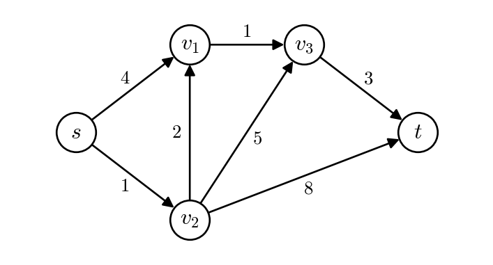
Exercise 8.1 (Dijkstra’s algorithm by hand) Apply Algorithm 1 to the directed graph in Figure 8.2 with start vertex s. Show d(v) after each iteration as in Table 8.1, and give the shortest path length from s to each vertex. Check your answer with dijkstra().

Code
G = nx.DiGraph()
G.add_weighted_edges_from([
    ("s", "v1", 4), ("s", "v2", 1), ("v2", "v1", 2), ("v1", "v3", 1),
    ("v2", "v3", 5), ("v3", "t", 3), ("v2", "t", 8),
])
pos = {"s": (0, 1), "v1": (1.3, 2), "v2": (1.3, 0), "v3": (2.6, 2), "t": (3.9, 1)}
draw_graph(G, pos, 4.5, 2.4)
A directed graph with five vertices drawn as circles labeled s, v1, v2, v3, and t. Vertex s is at the left, v1 and v3 are in the top row, v2 is in the bottom row, and t is at the right. The edges and their weights are s to v1 with weight 4, s to v2 with weight 1, v2 to v1 with weight 2, v1 to v3 with weight 1, v2 to v3 with weight 5, v3 to t with weight 3, and v2 to t with weight 8.
Figure 8.2: A directed graph with five vertices. The number on each edge is its weight.