29  Local Search

Consider the following optimization problem, where f is a real-valued objective function and \mathcal{X} is a nonempty finite feasible set:

\begin{aligned} \min \quad & f(\mathbf{x}) \\ \text{s.t.} \quad & \mathbf{x} \in \mathcal{X} \end{aligned}

Let N\colon \mathcal{X} \to 2^{\mathcal{X}} be a neighborhood mapping that assigns a set of neighboring feasible solutions N(\mathbf{x}) \subseteq \mathcal{X} to each solution \mathbf{x} \in \mathcal{X}. Define I(\mathbf{x}) as the set of neighboring solutions that have a better objective function value than \mathbf{x}, that is,

I(\mathbf{x}) = \{\mathbf{y} \in N(\mathbf{x}) : f(\mathbf{y}) < f(\mathbf{x})\}.

The algorithm starts from some initial solution \mathbf{x}^{(0)} \in \mathcal{X}. Then, it iteratively moves to any neighboring solution \mathbf{y} \in I(\mathbf{x}) such that f(\mathbf{y}) < f(\mathbf{x}). The algorithm terminates when there are no neighboring solutions with a better objective function value, i.e., when I(\mathbf{x}) = \emptyset. Since \mathcal{X} is finite and every move strictly decreases the objective function value, no solution can be revisited, so the algorithm terminates after finitely many moves. And finially, the algorithm can find a local optimum with respect to the neighborhood N. The general local search algorithm is given in Algorithm 1.

\begin{algorithm} \caption{Local Search} \begin{algorithmic} \Require initial solution $\mathbf{x}^{(0)} \in \mathcal{X}$, neighborhood $N$ \Ensure local optimum $\mathbf{x}$ with respect to $N$ \State $\mathbf{x} \gets \mathbf{x}^{(0)}$ \While{$I(\mathbf{x}) \neq \emptyset$} \State choose $\mathbf{y} \in I(\mathbf{x})$ \State $\mathbf{x} \gets \mathbf{y}$ \EndWhile \State \textbf{return} $\mathbf{x}$ \end{algorithmic} \end{algorithm}

The local search algorithm provides a simple and general framework for solving optimization problems. To implement the local search algorithm, we need to define

1. how to obtain an initial solution \mathbf{x}^{(0)},
2. how to define the neighborhood N of a solution, and
3. how to select a neighboring solution \mathbf{y} \in I(\mathbf{x}).

Those decisions are usually problem-specific and can significantly affect the performance of the algorithm. The initial solution can be obtained by randomly sampling from the feasible set \mathcal{X} or by using heuristics to construct a solution. The neighborhood is usually designed based on the structure of the problem.

Two common strategies for selecting a neighboring solution are the first-improvement and best-improvement strategies. The first-improvement strategy evaluates the neighbors in a fixed order and moves to the first one in I(\mathbf{x}). The best-improvement strategy evaluates all neighbors and moves to the one with the smallest f(\mathbf{y}) if I(\mathbf{x}) is not empty.

Previous research (Hansen and Mladenović 2006; Aloise et al. 2025) have conducted empirical studies on the performance of first-improvement and best-improvement strategies.

29.1 The Traveling Salesman Problem

In the Traveling Salesman Problem (TSP), we are given a set of nodes \{1, 2, \ldots, n\} and the distance d_{ij} between node i and node j. Assuming that the distance is symmetric, i.e., d_{ij} = d_{ji}, the n \times n distance matrix D = (d_{ij}) is symmetric. Define a tour \mathbf{x} = (x_1, x_2, \ldots, x_n) as a sequence of nodes that starts and ends at the same city and visits each city exactly once. The objective is to find a tour with minimal total length f(\mathbf{x}) = \sum_{k=1}^{n-1} d_{x_k x_{k+1}} + d_{x_n x_1}.

A permutation of a finite set is an ordered sequence in which each element of the set appears exactly once. We represent a tour by a permutation \mathbf{x} = (x_1,\ldots,x_n) of the cities, where x_k is the kth city visited. After visiting x_n, the tour returns to x_1. Thus, the feasible solution set is

\mathcal{X} = \{\mathbf{x} = (x_1, x_2, \ldots, x_n) : x_i \in \{1, 2, \ldots, n\}, x_i \neq x_j \text{ for } i \neq j\}.

29.1.1 Neighborhoods for the TSP

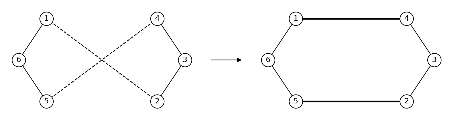
In the TSP, a well-known neighborhood is defined by the 2-opt exchange. Flood (1956) introduced the basic exchange idea, and Croes (1958) later developed a heuristic based on these exchanges. The 2-opt exchange removes two nonadjacent edges from the tour and replaces them with two different edges that form a new tour.

Example 29.1 (A 2-opt exchange) Consider the six-city tour \mathbf{x} = (1,2,3,4,5,6) shown in Figure 29.1. A 2-opt exchange replaces the edges \{1,2\} and \{4,5\} with \{1,4\} and \{2,5\}. This gives the new tour \mathbf{y} = (1,4,3,2,5,6).

import matplotlib.pyplot as plt

positions = {
    1: (0, 3),
    2: (4, 0),
    3: (5, 1.5),
    4: (4, 3),
    5: (0, 0),
    6: (-1, 1.5),
}
before = [1, 2, 3, 4, 5, 6]
after = before[:1] + before[1:4][::-1] + before[4:]
removed = {frozenset((1, 2)), frozenset((4, 5))}
added = {frozenset((1, 4)), frozenset((2, 5))}

fig, ax = plt.subplots(figsize=(9, 2.25))
for offset, tour, changed, style, width in [
    (0, before, removed, "--", 1.2),
    (9, after, added, "-", 2.5),
]:
    closed_tour = tour + tour[:1]
    for i, j in zip(closed_tour, closed_tour[1:]):
        start, end = positions[i], positions[j]
        is_changed = frozenset((i, j)) in changed
        ax.plot(
            [start[0] + offset, end[0] + offset],
            [start[1], end[1]],
            color="black",
            linestyle=style if is_changed else "-",
            linewidth=width if is_changed else 1.0,
            zorder=1,
        )

    for city, (x, y) in positions.items():
        ax.scatter(
            x + offset,
            y,
            s=390,
            color="white",
            edgecolor="black",
            linewidth=1.0,
            zorder=3,
        )
        ax.text(
            x + offset, y, str(city), ha="center", va="center", fontsize=11, zorder=4
        )

ax.annotate(
    "",
    xy=(7.1, 1.5),
    xytext=(5.9, 1.5),
    arrowprops=dict(arrowstyle="-|>", color="black", mutation_scale=14),
)
ax.set(xlim=(-1.5, 14.5), ylim=(-0.5, 3.5), aspect="equal")
ax.axis("off")
fig.subplots_adjust(left=0, right=1, top=1, bottom=0)
plt.show()

Figure 29.1: A 2-opt exchange. Dashed edges are removed, thick solid edges are added, and thin solid edges are unchanged.

This neighborhood can be generalized to the k-opt exchange, which removes k edges and adds k new edges to form a new tour. In particular, 3-opt (Lin 1965) can find improvements that 2-opt cannot, but its neighborhood is more expensive to search. A full scan considers O(n^3) triples of edges for 3-opt, compared with O(n^2) pairs for 2-opt (Snyder and Shen 2019, 437–38).

Formally, given a tour \mathbf{x} = (x_1, x_2, \ldots, x_n), we consider disjoint edges \{x_i, x_{i+1}\} and \{x_j, x_{j+1}\}, where i < j. The 2-opt exchange removes these two edges and adds the edges \{x_i, x_j\} and \{x_{i+1}, x_{j+1}\}. This gives a new tour

\mathbf{y} = (x_1, \ldots, x_i, x_j, x_{j-1}, \ldots, x_{i+1}, x_{j+1}, \ldots, x_n).

We can see that this operation reverses the segment (x_{i+1}, \ldots, x_j). In Example 29.1, i = 1 and j = 4, and the segment (2, 3, 4) is reversed.

Now we count the number of neighbors in the 2-opt neighborhood. The tour has n edges, and we choose two edges to conduct the 2-opt exchange. Since the selection order does not matter, there are \binom{n}{2} = n(n-1)/2 ways to choose two edges. Furthermore, edges such as \{x_i, x_{i+1}\} and \{x_{i+1}, x_{i+2}\}, and \{x_n, x_1\} and \{x_1, x_2\} are adjacent, so we do not consider them. There are n pairs of adjacent edges, so the number of pairs of nonadjacent edges is n(n-1)/2 - n = n(n-3)/2.

To apply the local search algorithm, we need to identify whether a 2-opt exchange improves the tour. Let \mathbf{x} be the current tour and \mathbf{y} be the tour after a 2-opt exchange. The change in the objective function is

f(\mathbf{y}) - f(\mathbf{x}) = d_{x_i x_j} + d_{x_{i+1} x_{j+1}} - d_{x_i x_{i+1}} - d_{x_j x_{j+1}}.

29.1.2 Python Implementation

The following two_opt_move() function implements the 2-opt exchange. Python uses zero-based indexing, so tour[k] corresponds to x_{k+1} in the mathematical notation above. The slice tour[i + 1 : j + 1][::-1] reverses the entries from tour[i + 1] through tour[j], corresponding to (x_{i+2}, \ldots, x_{j+1}). Thus, the mathematical indices i = 1 and j = 4 in Example 29.1 correspond to the Python arguments i = 0 and j = 3.

def two_opt_move(tour, i, j):
    """Remove edges {tour[i], tour[i+1]} and {tour[j], tour[(j+1) % len(tour)]},
    and reconnect the tour by reversing tour[i+1], ..., tour[j]."""
    return tour[: i + 1] + tour[i + 1 : j + 1][::-1] + tour[j + 1 :]

x = [1, 2, 3, 4, 5, 6]
print(two_opt_move(x, 0, 3))

[1, 4, 3, 2, 5, 6]

The difference in the tour length caused by a 2-opt exchange can be computed without computing the entire tour length. The following delta() function implements this calculation. When j + 1 = n, tour[(j + 1) % n] returns tour[0], which is the first city in the tour.

def delta(tour, i, j, D):
    """Change in the tour length caused by two_opt_move(tour, i, j)."""
    n = len(tour)
    a, b = tour[i], tour[i + 1]
    c, d = tour[j], tour[(j + 1) % n]
    return D[a, c] + D[b, d] - D[a, b] - D[c, d]

Using Python’s zero-based indices, the selected edges are adjacent when j = i + 1 or (i, j) = (0, n - 1). In the first case, the reversal leaves the list unchanged. In the second, it reverses the direction of traversal but preserves the same undirected edges and total length. We therefore exclude both cases. The generator two_opt_moves lists all n(n-3)/2 exchanges.

def two_opt_moves(n):
    """All 2-opt moves (i, j) for a tour of n cities."""
    for i in range(n - 2):
        for j in range(i + 2, n):
            if i == 0 and j == n - 1:
                continue  # {tour[0], tour[1]} and {tour[n-1], tour[0]} are adjacent
            yield i, j

x = [1, 2, 3, 4, 5, 6]
print(len(list(two_opt_moves(len(x)))))

9

Given a tour and the distance matrix, the following tour_length() function computes the total length of the tour.

def tour_length(tour, D):
    """Length of the tour, including the edge back to the first city."""
    return sum(D[tour[k - 1], tour[k]] for k in range(len(tour)))

29.1.3 Local Search with the 2-opt Neighborhood

With the 2-opt neighborhood, it remains to choose the initial tour and the strategy for selecting \mathbf{y} \in I(\mathbf{x}).

Here, we choose a random permutation of the cities as the initial tour. For the selection rule, we consider the first-improvement and best-improvement strategies.

The function local_search follows Algorithm 1. Its argument select is the selection rule, which can take the value first_improvement or best_improvement and returns a move (i, j) if there is an improving 2-opt exchange, or None if there is none.

def first_improvement(tour, D):
    """Return the first improving move, or None if there is none."""
    for i, j in two_opt_moves(len(tour)):
        if delta(tour, i, j, D) < 0:
            return i, j
    return None


def best_improvement(tour, D):
    """Return the move with the largest decrease, or None if there is none."""
    best_move, best_delta = None, 0
    for i, j in two_opt_moves(len(tour)):
        change = delta(tour, i, j, D)
        if change < best_delta:
            best_move, best_delta = (i, j), change
    return best_move


def local_search(tour, D, select):
    """2-opt local search. Return the local optimum and the tour lengths."""
    lengths = [tour_length(tour, D)]
    move = select(tour, D)
    while move is not None:  # while I(x) is not empty
        i, j = move
        tour = two_opt_move(tour, i, j)
        lengths.append(tour_length(tour, D))
        move = select(tour, D)
    return tour, lengths

29.1.4 The Car 54 Instance

We apply local search to a TSP with 33 cities in the United States, where d_{ij} is the road distance in miles between cities i and j. The distance table is from Karg and Thompson (1964); the table and the coordinates of the cities are available on the Road TSP History page of the University of Waterloo. The code below also stores the optimal tour for comparison. Note that the Car 54 instance uses road distances instead of Euclidean distances.

NoteThe 1962 Car 54 contest

In 1962, Procter & Gamble, a sponsor of the television series Car 54, Where Are You?, ran a contest with a $10,000 prize for the shortest tour through these 33 cities, using Rand McNally road distances. Robert Karg and Gerald Thompson of the Carnegie Institute of Technology designed a tour-finding method that ran on an electronic computer, and their tour tied for first place. The method did not guarantee optimality, but the tour reported in Karg and Thompson (1964) turned out to be optimal.

import numpy as np

# Name, latitude, and longitude of each city
cities = [
    ("Chicago, IL", 41.8500, -87.6500),
    ("Indianapolis, IN", 39.7667, -86.1500),
    ("Marion, OH", 40.5833, -83.1167),
    ("Erie, PA", 42.1167, -80.0833),
    ("Carlisle, PA", 40.2000, -77.1833),
    ("Wana, WV", 39.7000, -80.2833),
    ("Wilkesboro, NC", 36.1500, -81.1333),
    ("Chattanooga, TN", 35.0333, -85.3000),
    ("Barnwell, SC", 33.2333, -81.3500),
    ("Bainbridge, GA", 30.9000, -84.5667),
    ("Baton Rouge, LA", 30.4500, -91.1500),
    ("Little Rock, AR", 34.7333, -92.2833),
    ("Kansas City, MO", 39.0833, -94.5667),
    ("La Crosse, WI", 43.8000, -91.2333),
    ("Blunt, SD", 44.5000, -99.9833),
    ("Lincoln, NE", 40.8000, -96.6667),
    ("Wichita, KS", 37.6833, -97.3333),
    ("Amarillo, TX", 35.2167, -101.8167),
    ("Truth or Consequences, NM", 33.1167, -107.2500),
    ("Manuelito, NM", 35.4167, -108.9833),
    ("Colorado Springs, CO", 38.8333, -104.8167),
    ("Butte, MT", 46.0000, -112.5333),
    ("Lewiston, ID", 46.4167, -117.0167),
    ("Boise, ID", 43.6000, -116.2000),
    ("Twin Falls, ID", 42.5500, -114.4500),
    ("Salt Lake City, UT", 40.7500, -111.8833),
    ("Mexican Hat, UT", 37.1500, -109.8500),
    ("Marble Canyon, AZ", 36.8000, -111.6333),
    ("Reno, NV", 39.5167, -119.8000),
    ("Lone Pine, CA", 36.6000, -118.0500),
    ("Gustine, CA", 37.2500, -120.9833),
    ("Redding, CA", 40.5833, -122.3833),
    ("Portland, OR", 45.5167, -122.6667),
]

# Road distances in miles. Row i lists the distances from city i
# to cities 0, 1, ..., i - 1 (the lower triangle of D).
lower_triangle = [
    [184],
    [292, 195],
    [449, 310, 215],
    [670, 540, 380, 288],
    [516, 357, 232, 200, 211],
    [598, 514, 434, 566, 436, 381],
    [618, 434, 493, 787, 814, 642, 295],
    [881, 697, 719, 790, 632, 697, 224, 320],
    [909, 964, 955, 1020, 974, 952, 541, 341, 318],
    [978, 892, 1031, 1246, 1352, 1180, 843, 538, 747, 441],
    [654, 597, 803, 1018, 1154, 1104, 766, 461, 749, 634, 380],
    [504, 503, 722, 937, 1043, 806, 986, 722, 1042, 954, 784, 404],
    [276, 460, 568, 725, 946, 817, 874, 894, 1214, 1185, 1218, 660, 452],
    [780, 964, 1072, 1229, 1450, 1321, 1378, 1326, 1646, 1672, 1410, 1030, 626, 476],
    [529, 644, 789, 1004, 1184, 1001, 1214, 950, 1270, 1213, 1043, 632, 219, 436, 419],
    [805, 698, 917, 1132, 1238, 1055, 1113, 842, 1162, 1027, 779, 473, 195, 637, 634,
     256],
    [1181, 1007, 1226, 1441, 1547, 1364, 1375, 1080, 1134, 1138, 783, 611, 563, 1046,
     759, 624, 368],
    [1548, 1444, 1630, 1845, 1984, 1801, 1726, 1431, 1685, 1477, 1134, 1033, 906, 1389,
     1094, 967, 711, 404],
    [1547, 1454, 1668, 1883, 1994, 1811, 1879, 1584, 1776, 1632, 1267, 1053, 944, 1427,
     1196, 1005, 749, 442, 251],
    [1239, 1167, 1353, 1568, 1707, 1524, 1584, 1313, 1633, 1498, 1151, 979, 614, 988,
     600, 525, 471, 368, 512, 507],
    [1538, 1733, 1830, 2045, 2208, 2090, 2136, 2078, 2398, 2332, 2110, 1782, 1378, 1300,
     760, 1229, 1382, 1319, 1163, 930, 910],
    [1999, 2158, 2291, 2448, 2669, 2515, 2597, 2500, 2820, 2675, 2336, 2164, 1707, 1860,
     1375, 1582, 1658, 1545, 1389, 1156, 1237, 436],
    [1716, 1875, 2008, 2165, 2386, 2232, 2488, 2217, 2537, 2392, 2053, 1881, 1422, 1577,
     1106, 1244, 1375, 1262, 1106, 873, 954, 483, 283],
    [1580, 1738, 1872, 2029, 2250, 2095, 2352, 2081, 2401, 2256, 1917, 1745, 1286, 1473,
     988, 1147, 1239, 1126, 970, 737, 818, 379, 419, 136],
    [1425, 1569, 1717, 1874, 2109, 1926, 2115, 1844, 2164, 2019, 1680, 1508, 1118, 1335,
     862, 913, 1002, 889, 733, 500, 581, 430, 656, 373, 237],
    [1560, 1549, 1852, 2009, 2089, 1906, 2063, 1792, 2112, 1967, 1456, 1274, 1032, 1540,
     1068, 1007, 944, 665, 521, 282, 491, 768, 994, 711, 575, 358],
    [1918, 1744, 1963, 2178, 2284, 2101, 2174, 1879, 2071, 1892, 1562, 1348, 1239, 1722,
     1258, 1300, 1044, 737, 526, 295, 802, 816, 1022, 739, 603, 386, 545],
    [2065, 2102, 2357, 2514, 2642, 2459, 2626, 2355, 2675, 2530, 2191, 2019, 1673, 1905,
     1432, 1570, 1507, 1320, 1109, 878, 1124, 842, 715, 432, 465, 533, 849, 739],
    [2284, 2131, 2326, 2441, 2671, 2488, 2418, 2133, 2437, 2259, 1929, 1715, 1606, 1924,
     1451, 1589, 1411, 1104, 893, 662, 1143, 1004, 981, 698, 599, 589, 768, 523, 266],
    [2340, 2348, 2543, 2658, 2888, 2705, 2869, 2598, 2918, 2773, 2434, 2262, 1916, 2148,
     1675, 1813, 1750, 1468, 1102, 871, 1367, 1085, 958, 675, 1033, 778, 1092, 982, 243,
     349],
    [2247, 2327, 2539, 2696, 2867, 2684, 2851, 2580, 2900, 2755, 2416, 2244, 1898, 2130,
     1657, 1795, 1732, 1545, 1334, 1103, 1349, 1014, 814, 531, 1015, 760, 1047, 964,
     225, 497, 266],
    [2163, 2322, 2455, 2612, 2833, 2679, 2761, 2664, 2984, 2839, 2500, 2328, 1871, 2024,
     1539, 1746, 1822, 1709, 1553, 1320, 1391, 693, 346, 447, 583, 820, 1158, 1355, 581,
     847, 710, 444],
]

n = len(cities)
D = np.zeros((n, n), dtype=int)
for i, row in enumerate(lower_triangle, start=1):
    D[i, :i] = row
D = D + D.T

# The optimal tour reported by Karg and Thompson (1964)
optimal_tour = [0, 1, 2, 3, 5, 4, 6, 8, 7, 9, 10, 11, 12, 15, 16, 17, 18,
                19, 27, 29, 28, 30, 31, 32, 22, 23, 24, 21, 25, 26, 20, 14, 13]
optimal_length = tour_length(optimal_tour, D)

We start both selection rules from the same random tour.

rng = np.random.default_rng(0)
initial_tour = rng.permutation(n).tolist()

tour_first, lengths_first = local_search(initial_tour, D, first_improvement)
tour_best, lengths_best = local_search(initial_tour, D, best_improvement)

print(f"Initial tour:      {lengths_first[0]:,} miles")
print(f"First improvement: {lengths_first[-1]:,} miles after {len(lengths_first) - 1} moves")
print(f"Best improvement:  {lengths_best[-1]:,} miles after {len(lengths_best) - 1} moves")
print(f"Optimal tour:      {optimal_length:,} miles")

Initial tour:      42,650 miles
First improvement: 11,033 miles after 84 moves
Best improvement:  11,369 miles after 32 moves
Optimal tour:      10,861 miles

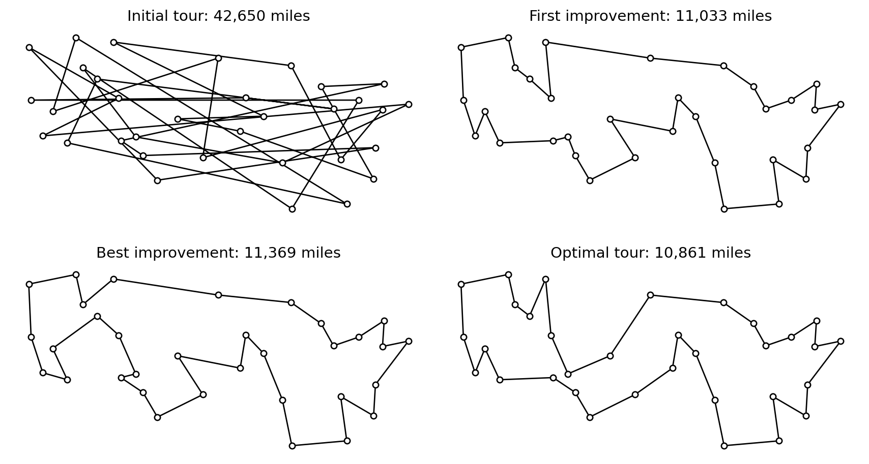
Figure 29.2 shows the initial tour, the tours found by local search with the two selection methods, and the optimal tour. In this experiment, both methods find a local optimum, but neither method finds the optimal tour. First improvement finds a shorter tour than best improvement.

lon = np.array([city[2] for city in cities])
lat = np.array([city[1] for city in cities])
panels = [
    (initial_tour, "Initial tour"),
    (tour_first, "First improvement"),
    (tour_best, "Best improvement"),
    (optimal_tour, "Optimal tour"),
]

fig, axes = plt.subplots(2, 2, figsize=(9, 5.2))
for ax, (tour, title) in zip(axes.flat, panels):
    closed_tour = tour + tour[:1]
    ax.plot(lon[closed_tour], lat[closed_tour], color="black", linewidth=1, zorder=1)
    ax.scatter(lon, lat, s=18, color="white", edgecolor="black", zorder=2)
    ax.set_title(f"{title}: {tour_length(tour, D):,} miles", fontsize=11)
    # One degree of longitude is shorter than one degree of latitude
    ax.set_aspect(1 / np.cos(np.radians(lat.mean())))
    ax.axis("off")
fig.tight_layout()
plt.show()

Figure 29.2: Tours for the Car 54 instance. The local search starts from the random initial tour.

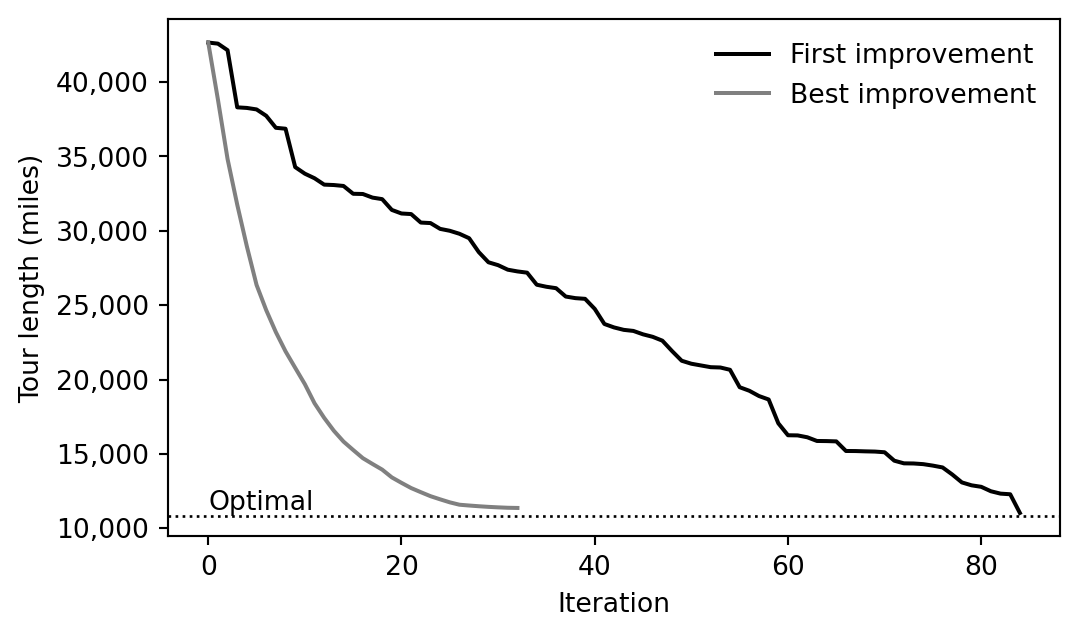
Figure 29.3 shows the tour length at each iteration. In this experiment, best improvement reduces the tour length more rapidly over the early iterations and terminates after 32 moves, compared with 84 for first improvement. However, best improvement scans the entire neighborhood at each iteration, while first improvement stops scanning as soon as it finds an improving move. Best improvement therefore typically evaluates more neighbors per iteration.

from matplotlib.ticker import StrMethodFormatter

fig, ax = plt.subplots(figsize=(6, 3.5))
ax.plot(lengths_first, color="black", label="First improvement")
ax.plot(lengths_best, color="gray", label="Best improvement")
ax.axhline(optimal_length, color="black", linestyle=":", linewidth=1)
ax.text(0, optimal_length, "Optimal", va="bottom")
ax.yaxis.set_major_formatter(StrMethodFormatter("{x:,.0f}"))
ax.set_xlabel("Iteration")
ax.set_ylabel("Tour length (miles)")
ax.legend(frameon=False)
plt.show()

Figure 29.3: Tour length at each iteration, starting from the initial tour in Figure 29.2.

29.2 Multi-Start Local Search

Different initial solutions can lead to different local optima. Multi-start local search runs local search from several initial solutions and keeps the best solution found. Algorithm 2 describes this strategy for the general optimization problem introduced at the beginning of this chapter.

\begin{algorithm} \caption{Multi-Start Local Search} \begin{algorithmic} \Require objective function $f$, neighborhood $N$, number of starts $R \geq 1$ \Ensure best solution found $\mathbf{x}_{\text{best}}$ \State $f_{\text{best}} \gets +\infty$ \For{$r = 1, \ldots, R$} \State generate an initial solution $\mathbf{x}^{(0)} \in \mathcal{X}$ \State $\mathbf{x} \gets$ \textsc{LocalSearch}$(\mathbf{x}^{(0)}, N)$ \If{$f(\mathbf{x}) < f_{\text{best}}$} \State $\mathbf{x}_{\text{best}} \gets \mathbf{x}$ \State $f_{\text{best}} \gets f(\mathbf{x})$ \EndIf \EndFor \State \textbf{return} $\mathbf{x}_{\text{best}}$ \end{algorithmic} \end{algorithm}

For the Car 54 instance, we use first improvement and R = 100 random initial tours. The variables best_tour and best_length store the best result so far. We also record the length of each local optimum in final_lengths to see how the results vary.

n_starts = 100
rng = np.random.default_rng(0)
best_tour = None
best_length = float("inf")
final_lengths = []

for _ in range(n_starts):
    random_tour = rng.permutation(n).tolist()
    tour, lengths = local_search(random_tour, D, first_improvement)
    length = lengths[-1]
    final_lengths.append(length)
    if length < best_length:
        best_tour = tour
        best_length = length

print(f"Best of {n_starts:,} starts: {best_length:,} miles")
print(f"Optimal tour:         {optimal_length:,} miles")

Best of 100 starts: 10,861 miles
Optimal tour:         10,861 miles

Figure 29.4 shows the results of the multi-start local search. The circles show the length returned by each local search, and the step line shows the best length found so far. In this experiment, the first start gives 11,033 miles, and the second reaches the known optimum of 10,861 miles. Later starts can give longer tours, but the best tour is retained.

n_shown = 100
starts = np.arange(1, n_shown + 1)
values = np.array(final_lengths[:n_shown])
best_so_far = np.minimum.accumulate(values)

fig, ax = plt.subplots(figsize=(7, 3.8))
ax.step(starts, best_so_far, where="post", color="black", linewidth=1.5, zorder=1)
ax.scatter(starts, values, s=15, color="white", edgecolor="black", zorder=2)
status = " (optimal)" if best_length == optimal_length else ""
ax.set_title(f"Best of {n_starts} starts: {best_length:,} miles{status}", fontsize=11)
ax.set_xlim(0.5, n_shown + 1)
ax.set_ylim(optimal_length - 180, values.max() + 120)
ax.set_xticks([1, 20, 40, 60, 80, 100])
ax.set_xlabel("Start number")
ax.set_ylabel("Local optimum length (miles)")
ax.yaxis.set_major_formatter(StrMethodFormatter("{x:,.0f}"))
ax.spines[["top", "right"]].set_visible(False)
fig.tight_layout()
plt.show()

Figure 29.4: Results of 100 starts using first improvement. Individual results vary, while the best tour length found so far never increases. It reaches the known optimal length at start 2.

More starts require more computation and give more opportunities to find a better solution, but still do not guarantee finding the optimal solution.

29.3 Related Materials

The following references provide additional information on local search.

• Combinatorial Optimization: Algorithms and Complexity, by Christos H. Papadimitriou and Kenneth Steiglitz
• Introduction to Linear Optimization, by Dimitris Bertsimas and John N. Tsitsiklis

The following references provide additional information on the TSP and the local search algorithm.

• Fundamentals of Supply Chain Theory, by Lawrence V. Snyder and Zuo-Jun Max Shen

29.4 Exercises

Exercise 29.1 (2-opt by Hand) Consider a TSP with five cities and the distances d_{ij} in Table 29.1.

Table 29.1: Distances d_{ij} between the five cities.

	1	2	3	4	5
1	0	6	3	9	8
2	6	0	6	6	7
3	3	6	0	6	9
4	9	6	6	0	3
5	8	7	9	3	0

Start the local search from the tour \mathbf{x} = (1, 2, 3, 4, 5).

1. List the 2-opt neighbors of \mathbf{x}, and compute f(\mathbf{y}) - f(\mathbf{x}) for each neighbor \mathbf{y}.
2. Suppose that first improvement scans the exchanges in the order (i, j) = (1, 3), (1, 4), (2, 4), (2, 5), (3, 5), which is the order used by two_opt_moves. Which neighbor does first improvement choose? Which neighbor does best improvement choose?
3. Continue each local search until it terminates. Report the local optimum and its length for each selection rule.
4. Different permutations can represent the same tour. How many distinct tours are there for five cities? Find an optimal tour by enumerating them. Is either local optimum optimal?

Exercise 29.2 (Constructing an Initial Tour) The local search in this chapter starts from a random tour, which is 42,650 miles long for the Car 54 instance.

1. Propose a method that constructs a short tour from the distance matrix D, and describe it in words or in pseudocode. (Hint: How would you plan a trip through the 33 cities by hand?)
2. Implement your method in Python, and report the length of the tour it constructs for the Car 54 instance.
3. Run the local search from your tour with first improvement and with best improvement. Compare the lengths of the local optima and the numbers of moves with those obtained from the random tour.
4. Multi-start local search needs many different initial solutions. How can your method generate different initial tours?

Exercise 29.3 (Local Search for the 0-1 Knapsack Problem) In the 0-1 knapsack problem, we are given n items and a knapsack with capacity K. Item j has a weight w_j and a value c_j. Let x_j = 1 if item j is put in the knapsack and x_j = 0 otherwise. The problem is

\begin{alignedat}{2} \max \quad & \sum_{j=1}^{n} c_j x_j \\ \text{s.t.} \quad & \sum_{j=1}^{n} w_j x_j \leq K \\ & x_j \in \{0, 1\}, &\qquad& j = 1, \ldots, n \end{alignedat}

Consider the instance in Table 29.2 with K = 15. Its optimal solution is \mathbf{x}^* = (1, 1, 0, 1) with total value 8, which is found by dynamic programming in Example 15.3.

Table 29.2: The weights and values of the items.

Item j	Weight w_j	Value c_j
1	12	4
2	2	2
3	1	1
4	1	2

1. Propose a local search for the 0-1 knapsack problem. Specify the feasible set \mathcal{X}, an initial solution, a neighborhood N with N(\mathbf{x}) \subseteq \mathcal{X}, and a selection rule. Note that this is a maximization problem, and that, unlike a 2-opt exchange in the TSP, a small change to a feasible solution may violate the constraint.
2. Apply your local search to the instance by hand. Does it find the optimal solution?
3. In the flip neighborhood, a neighbor is a feasible solution obtained by adding one item to the knapsack or removing one item from it. Show that (1, 1, 1, 0) is a local optimum with respect to the flip neighborhood but is not optimal. Then propose a neighborhood with respect to which (1, 1, 1, 0) is not a local optimum.

Aloise, Daniel, Robin Moine, Celso C Ribeiro, and Jonathan Jalbert. 2025. “First-Improvement or Best-Improvement? An in-Depth Local Search Computational Study to Elucidate a Dominance Claim.” European Journal of Operational Research 326 (3): 413–26. https://doi.org/10.1016/j.ejor.2025.04.019.

Croes, G. A. 1958. “A Method for Solving Traveling-Salesman Problems.” Operations Research 6 (6): 791–812. https://doi.org/10.1287/opre.6.6.791.

Flood, Merrill M. 1956. “The Traveling-Salesman Problem.” Operations Research 4 (1): 61–75. https://doi.org/10.1287/opre.4.1.61.

Hansen, Pierre, and Nenad Mladenović. 2006. “First Vs. Best Improvement: An Empirical Study.” Discrete Applied Mathematics (Amsterdam, Netherlands: 1988) 154 (5): 802–17. https://doi.org/10.1016/j.dam.2005.05.020.

Karg, Robert L, and Gerald L Thompson. 1964. “A Heuristic Approach to Solving Travelling Salesman Problems.” Management Science 10 (2): 225–48. https://doi.org/10.1287/mnsc.10.2.225.

Lin, Shen. 1965. “Computer Solutions of the Traveling Salesman Problem.” The Bell System Technical Journal 44 (10): 2245–69. https://doi.org/10.1002/j.1538-7305.1965.tb04146.x.

Snyder, Lawrence V, and Zuo-Jun Max Shen. 2019. Fundamentals of Supply Chain Theory. 2nd ed. John Wiley & Sons.