データサイエンスの分野では,最適化は非常に重要な役割を果たしている.最適化はある目的関数 \(f(\mathbf{x})\) を最小化または最大化する \(\mathbf{x}\) を求める問題である.一般的に,最適化問題は下記のように定式化される.
\[\begin{align*}
\text{minimize} \quad & f(\mathbf{x}) \\
\text{subject to} \quad & g_i(\mathbf{x}) \leq 0, \quad i = 1, \ldots, m \\
& h_j(\mathbf{x}) = 0, \quad j = 1, \ldots, p
\end{align*}\]
ここで,\(f\), \(g_i\), \(h_j\) は \(\mathbf{x} \in \mathbb{R}^n\) に関する関数である.特に,\(f\) は目的関数,\(g_i\),\(h_j\) は制約条件と呼ぶ.
\(\mathbf{x}\) は決定変数と呼ばれ,最適化問題の解ともいう.最適解は,目的関数の値が最小(または最大)となる決定変数の値であり,\(\mathbf{x}^*\) と表されることが多い.
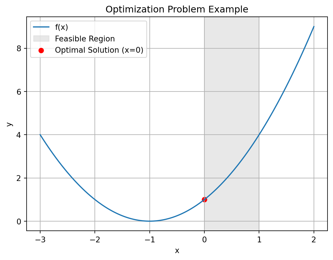
Example 15.1 (最適化問題の例) 次の最適化問題を考える.
\[\begin{align*}
\text{minimize} \quad & f(x) = x^2 + 2x + 1 \\
\text{subject to} \quad & x - 1 \leq 0 \\
& -x \leq 0
\end{align*}\]
import numpy as np
import matplotlib.pyplot as plt


def f(x):
    return x**2 + 2 * x + 1


x = np.linspace(-3, 2, 1000)
plt.plot(x, f(x), label="f(x)")
plt.title("Optimization Problem Example")
plt.xlabel("x")
plt.ylabel("y")
plt.axvspan(0, 1, color="lightgray", alpha=0.5, label="Feasible Region")
plt.scatter(0, f(0), color="red", label="Optimal Solution (x=0)")
plt.legend()
plt.grid()
plt.show()