import numpy as np

def calculate_rse(y_true, y_pred, p):
    n = len(y_true)
    rss = np.sum((y_true - y_pred) ** 2)
    rse = np.sqrt(rss / (n - p - 1))
    return rse

def calculate_r2(y_true, y_pred):
    tss = np.sum((y_true - np.mean(y_true)) ** 2)
    rss = np.sum((y_true - y_pred) ** 2)
    r2 = (tss - rss) / tss
return r214 モデルの精度
回帰モデルの精度を評価するには,以下の指標を用いることが一般的である。
- 残差標準誤差 (Residual Standard Error; RSE)
- 決定係数 (Coefficient of Determination; \(R^2\))
14.1 残差標準誤差
回帰モデルには,誤差項 \(\epsilon\) が含まれている.RSE は,この誤差項の標準偏差を推定するものであり,以下の式で計算される。
\[ \text{RSE} = \sqrt{\frac{1}{n - p - 1} \sum_{i=1}^{n} (y_i - \hat{y}_i)^2} = \sqrt{\frac{\text{RSS}}{n - p - 1}} \]
\(p\) は説明変数の数を表す.単回帰分析の場合,\(p=1\) である。RSS (残差平方和; Residual Sum of Squares)は以下の式で計算される。
\[ \text{RSS} = \sum_{i=1}^{n} (y_i - \hat{y}_i)^2 \]
RSE が小さいほど,モデルの予測が観測値に近いことを示す.
RSE は,モデルの精度を評価するために用いられるが,\(Y\) のスケールに依存するため,決定係数がよく用いられる。
14.2 決定係数
決定係数 \(R^2\) は,モデルの精度を評価するための指標であり,0 から 1 の範囲で値を取る.
\(R^2\) は以下の式で計算される。
\[ R^2 = \frac{\text{TSS} - \text{RSS}}{\text{TSS}} \]
TSS (総平方和; Total Sum of Squares)は以下の式で計算される。
\[ \text{TSS} = \sum_{i=1}^{n} (y_i - \bar{y})^2 \]
TSS は,観測値 \(y_i\) とその平均 \(\bar{y}\) のばらつきを表す.\(\text{TSS} - \text{RSS}\) は,モデルが説明できるばらつきを表す.
すべての \(i\) について \(\hat{y}_i = y_i\) の場合,\(\text{RSS} = 0\) となり,\(R^2 = 1\) となる.一方,すべての \(i\) について \(\hat{y}_i = \bar{y}\) の場合,\(\text{RSS} = \text{TSS}\) となり,\(R^2 = 0\) となる.
\(R^2\) が 1 に近いほど,モデルの精度が高いことを示す.\(R^2\) が 0 に近い場合,モデルの精度が低いことを示す.
14.3 実装
14.4 Python による計算例
import numpy as np
from sklearn.linear_model import LinearRegression
from sklearn.metrics import r2_score
import matplotlib.pyplot as plt

# サンプルデータの生成
np.random.seed(0)
X = 2 * np.random.rand(100, 1)
y = 4 + 3 * X + np.random.randn(100, 1)

# 線形回帰モデルの学習
model = LinearRegression()
model.fit(X, y)

# plot
plt.scatter(X, y, color="blue")
plt.plot(X, model.predict(X), color="red")
plt.xlabel("X")
plt.ylabel("y")
plt.show()

# 決定係数の計算
r2 = r2_score(y, model.predict(X))
print(f"決定係数 R^2: {r2}")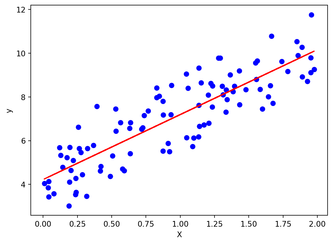
決定係数 R^2: 0.7469629925504755import numpy as np
from sklearn.linear_model import LinearRegression
from sklearn.metrics import r2_score
import matplotlib.pyplot as plt
# サンプルデータの生成
np.random.seed(0)
X = 2 * np.random.rand(100, 1)
y = 4 + 3 * X + 0.1 * np.random.randn(100, 1)
# 線形回帰モデルの学習
model = LinearRegression()
model.fit(X, y)
# plot
plt.scatter(X, y, color="blue")
plt.plot(X, model.predict(X), color="red")
plt.xlabel("X")
plt.ylabel("y")
plt.show()
# 決定係数の計算
r2 = r2_score(y, model.predict(X))
print(f"決定係数 R^2: {r2}")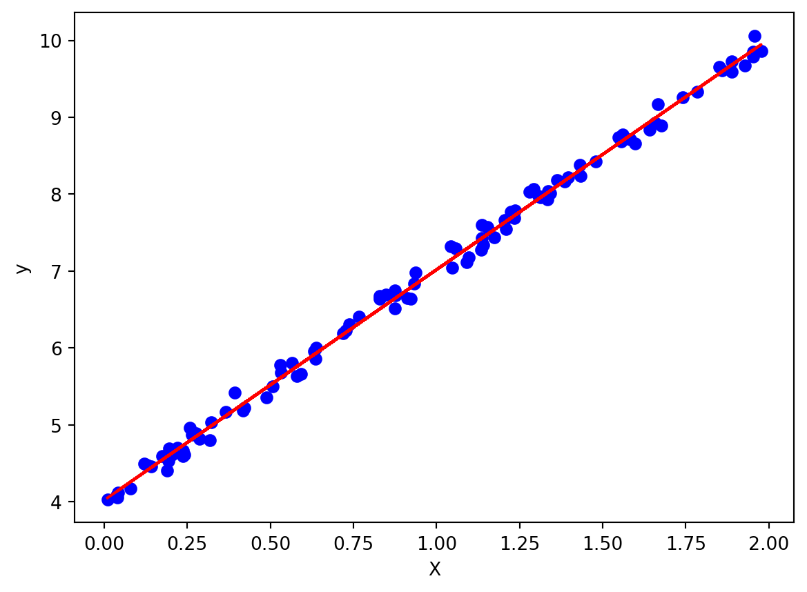
決定係数 R^2: 0.9966873204996887