1  Multi-armed Bandits

1.1 Introduction

The multi-armed bandit problem is a classic problem in which a decision-maker chooses between \(k\) different actions, each of which has an unknown reward distribution. After each action, the decision-maker receives a reward from a stationary probability distribution. The objective is to maximize the total reward over some time period.

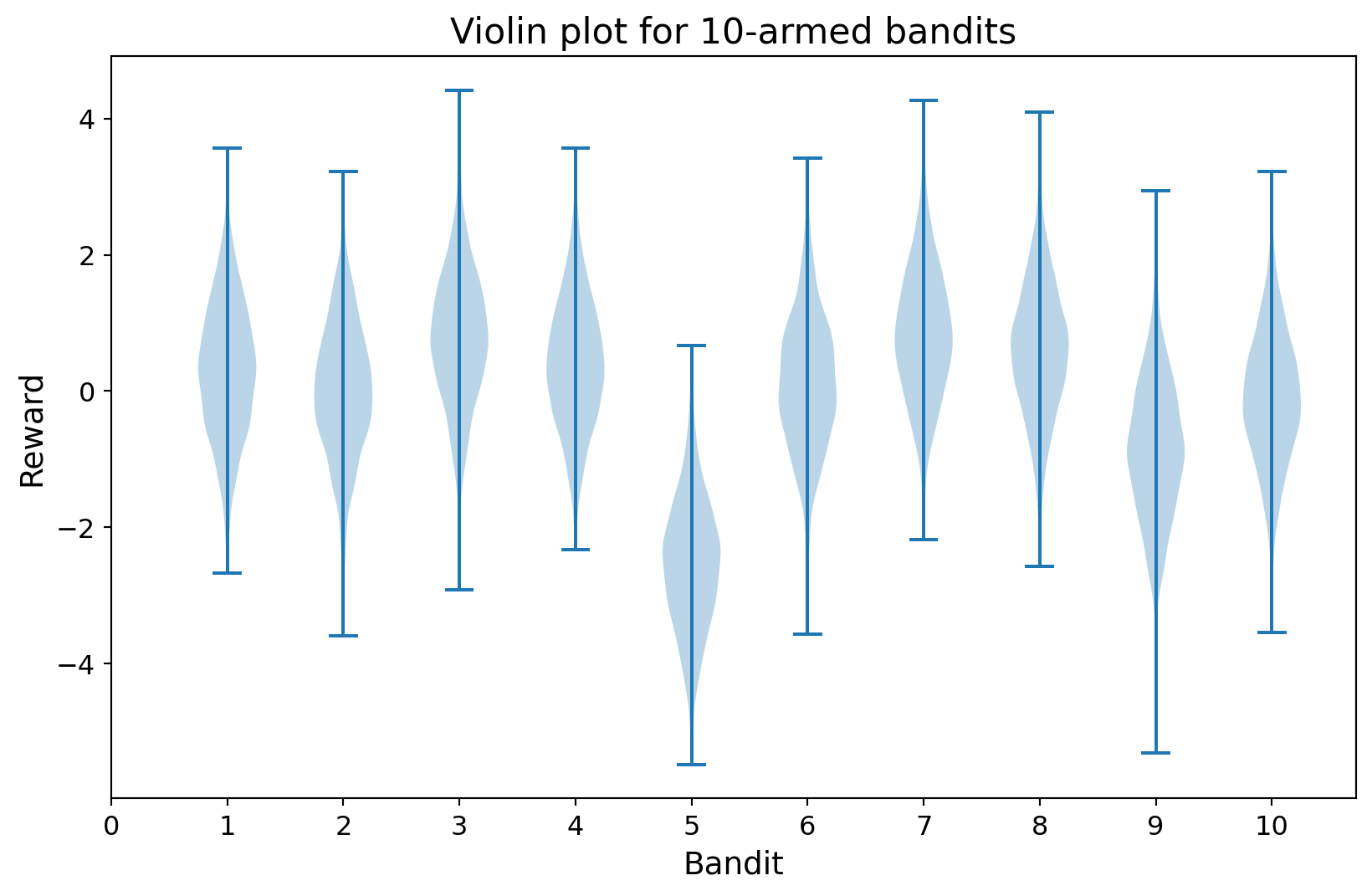
import numpy as np
import matplotlib.pyplot as plt

# Set the random seed for reproducibility
np.random.seed(0)

# Set the figure size
plt.figure(figsize=(10, 6))

# Generate the data and plot the violin plot
data = np.random.randn(2000, 10) + np.random.randn(10)
plt.violinplot(dataset=data)

# Set the labels and title with increased font sizes
plt.xlabel("Bandit", fontsize=14)
plt.ylabel("Reward", fontsize=14)
plt.title("Violin plot for 10-armed bandits", fontsize=16)

plt.tick_params(axis="both", which="major", labelsize=12)
plt.xticks(np.arange(0, 11))

# Save the figure
plt.show()

1.2 Notation

• \(A_t\): Action at time \(t\)
• \(R_t\): Reward at time \(t\)
• \(q_*(a)\): Expected reward for taking action \(a\)
• \(Q_t(a)\): Estimated value of action \(a\) at time \(t\)

1.3 Expected Reward and Estimated reward

Let \(q_*(a)\) be the expected reward for taking action \(a\), i.e., \(q_*(a) = \mathbb{E} \left[ R_t | A_t = a \right]\). Note that if \(q_*(a)\) is known, the optimal action is always to choose \(a = \arg \max_a q_*(a)\). However, since the reward distribution is unknown, we cannot directly compute \(q_*(a)\). Thus, we need to find a way to estimate \(q_*(a)\).

Let \(Q_t(a)\) be the estimated value of action \(a\) at time \(t\). A simple idea is to use the sample average of rewards obtained from action \(a\) up to time \(t-1\):

\[ Q_t(a) = \frac{\sum_{i=1}^{t-1} R_i \mathbb{I} \left\{ A_i = a \right\}}{\sum_{i=1}^{t-1} \mathbb{I} \left\{ A_i = a \right\}} \]

where \(\mathbb{I} \left\{ A_i = a \right\}\) is an indicator function that is equal to 1 if \(A_i = a\) and 0 otherwise.

As long as we obtain sufficient samples, the sample average will converge to the true expected reward. However, this method requires storing all the rewards and actions, which will be increasingly expensive as the number of actions and time steps increases.

1.4 Incremental Implementation

To avoid storing all the rewards and actions, we can use an incremental implementation of the sample average. The incremental implementation updates the estimated value of action \(a\) at time \(t\) using the following formula:

\[ Q_{n+1} = Q_n + \frac{1}{n} \left( R_n - Q_n \right) \]

where \(n\) is the number of times action \(a\) has been taken, \(R_n\) is the reward obtained after taking action \(a\) for the \(n\)-th time, and \(Q_n\) is the estimated value of action \(a\) after taking action \(a\) for the \(n\)-th time.

It is easy to prove that the incremental implementation is equivalent to the sample average implementation. The proof is as follows:

\[\begin{align*} Q_{n+1} & = \frac{R_1 + R_2 + \dots + R_{n}}{n} \\ & = \frac{1}{n} \sum_{i=1}^{n} R_i \\ & = \frac{1}{n} \left( R_n + \sum_{i=1}^{n-1} R_i \right) \\ & = \frac{1}{n} \left( R_n + (n-1) \frac{R_1 + R_2 + \dots + R_{n-1}}{n-1} \right) \\ & = \frac{1}{n} \left( R_n + (n-1) Q_n \right) \\ & = Q_n + \frac{1}{n} \left( R_n - Q_n \right) \\ \end{align*}\]

We can see that the incremental implementation is only required to store the estimated value \(Q_n\) and the number of times \(n\) for each action.

Now, we can use the incremental implementation to estimate the expected reward for each action. The next question is how to choose the action in each period.

1.5 Exploration and Exploitation

Remember that the objective of the multi-armed bandit problem is to maximize the total reward over some time period. To achieve this objective, we need to (1) explore the environment to estimate \(q_*(a)\) and (2) exploit the estimated values to maximize the total reward.

Should we equally explore all actions as much as possible to estimate \(q_*(a)\) accurately, or should we exploit the action with the highest estimated value to maximize the total reward? This is known as the exploration-exploitation dilemma.

The \(\epsilon\)-greedy policy is a simple policy that balances exploration and exploitation. In this policy, \(\epsilon\) is the probability that within the range \([0, 1]\). With probability \(\epsilon\), the agent chooses a random action (explore), and with probability \(1-\epsilon\), the agent chooses the action with the highest estimated value (exploit). Normally, \(\epsilon\) is set to a small value, such as 0.1 or 0.01.

1.6 A Simple Bandit Algorithm

We have discussed the methods to estimate the expected reward and to select the action. Now, we can combine these methods to create a simple bandit algorithm. The pseudocode is as follows:

\begin{algorithm} \caption{A Simple Bandit Algorithm} \begin{algorithmic} \For{$a = 1, 2, \dots, k$} \State $Q(a) \leftarrow 0$ \State $N(a) \leftarrow 0$ \EndFor \For{$t = 1, 2, \dots, T$} \State Choose $A_t$ using the $\epsilon$-greedy policy based on $Q$ \State $R_t \leftarrow \texttt{bandit}(A_t)$ \State $N(A_t) \leftarrow N(A_t) + 1$ \State $Q(A_t) \leftarrow Q(A_t) + \frac{1}{N(A_t)} \left( R_t - Q(A_t) \right)$ \EndFor \end{algorithmic} \end{algorithm}

In the beginning, we initialize the estimated value \(Q_t(a)\) and the number of times \(N_t(a)\) for each action to 0. In each period \(t\), we choose the action \(A_t\) using the \(\epsilon\)-greedy policy. After taking action \(A_t\), we receive the reward \(R_t\) and update the number of times \(N_t(A_t)\) . Then, we update the estimated value \(Q_t(A_t)\) using the incremental implementation.

1.7 Python Implementation

1.7.1 Multi-armed Bandit Problem

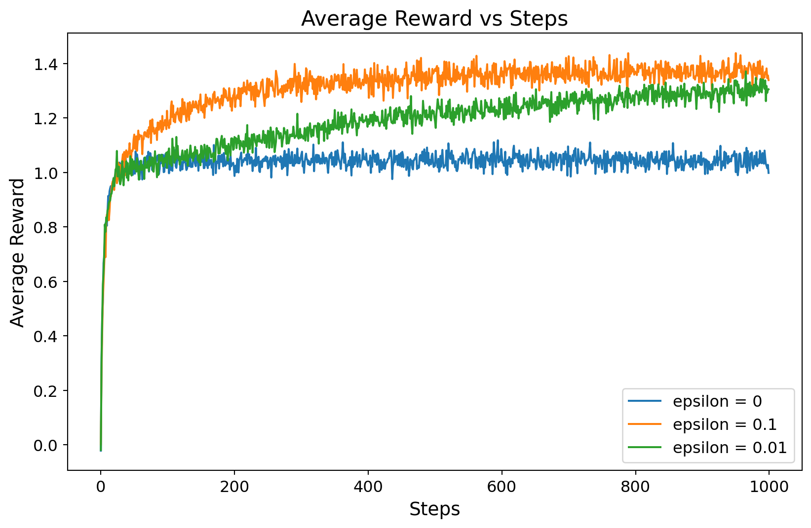
import numpy as np
import matplotlib.pyplot as plt


class bandit_algorithm:
    def __init__(self, bandit, epsilon, steps):
        self.bandit = bandit
        self.epsilon = epsilon
        self.steps = steps
        self.k = bandit.k
        self.Q = np.zeros(self.k)
        self.N = np.zeros(self.k)
        self.reward = np.zeros(self.steps)

    def learn(self):
        for t in range(self.steps):
            # epsilon greedy
            if np.random.rand() < self.epsilon:
                action = np.random.randint(self.k)
            else:
                # choose action with maximum Q, if multiple, choose randomly
                action = np.random.choice(np.where(self.Q == np.max(self.Q))[0])
            # get reward
            reward = self.bandit.bandit(action)
            # update Q
            self.N[action] += 1
            self.Q[action] += (reward - self.Q[action]) / self.N[action]
            # update reward
            self.reward[t] = reward


class bandit:
    def __init__(self, k):
        self.k = k
        self.mu = np.random.randn(k)
        self.sigma = np.ones(k)

    def bandit(self, action):
        return np.random.normal(self.mu[action], self.sigma[action])


if __name__ == "__main__":

    # set random seed for reproducibility
    np.random.seed(0)

    k = 10
    steps = 1000
    epsilon_list = [0, 0.1, 0.01]

    # mean reward
    number_of_runs = 2000
    rewards = np.zeros((len(epsilon_list), number_of_runs, steps))

    for i, epsilon in enumerate(epsilon_list):
        for j in range(number_of_runs):
            bandit_instance = bandit(k)
            simple_bandit = bandit_algorithm(bandit_instance, epsilon, steps)
            simple_bandit.learn()
            rewards[i, j, :] = simple_bandit.reward

    # plot
    plt.figure(figsize=(10, 6))
    for i in range(len(epsilon_list)):
        plt.plot(
            np.mean(rewards[i, :, :], axis=0),
            label="epsilon = {}".format(epsilon_list[i]),
        )
    plt.xlabel("Steps", fontsize=14)
    plt.ylabel("Average Reward", fontsize=14)
    plt.title("Average Reward vs Steps", fontsize=16)
    plt.tick_params(axis="both", which="major", labelsize=12)
    plt.legend(fontsize=12)
    plt.show()

1.7.2 The Newsvendor Problem

The newsvendor problem is a classic inventory management problem in which a decision-maker must decide how many copies of a newspaper to order each morning. The demand for the newspaper follows a probability distribution. The overage cost occurs when the demand is less than the order quantity, and the underage cost occurs when the demand is greater than the order quantity.

Note that the classic newsvendor problem assumes that the demand distribution is known and by minimizing the expected cost, we can find the optimal order quantity.

In here, we assume that the demand distribution is unknown, and we can only observe the demand after ordering the newspaper. The objective is to minimize the cost over some time period. By considering the discrete order quantity as actions, we can model the newsvendor problem as a multi-armed bandit problem.

Symbol	Description
\(D_t\)	Demand at time \(t\)
\(h\)	Holding cost (overage cost)
\(p\)	Stockout cost (underage cost)

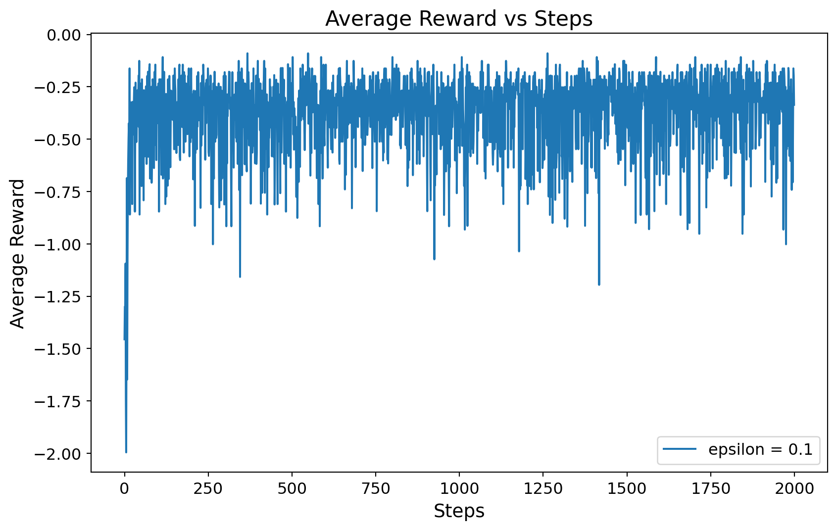
In the following code, we solve an instance of the newsvendor problem using the simple bandit algorithm. In this example, \(h = 0.18\), \(p = 0.7\), and \(D \sim \mathcal{N}(5, 1)\), where \(D\) is discretized to the nearest integer.

We set the planning horizon steps = 2000. We use the \(\epsilon\)-greedy policy with \(\epsilon = 0.1\). We run the algorithm 10 times by setting number_of_runs = 10 and store the results in the rewards array. Finally, we plot the average reward over time.

import numpy as np
import matplotlib.pyplot as plt


class newsvendor_as_bandits:
    def __init__(self, k, h, p, mu, sigma):
        self.k = k
        self.h = h
        self.p = p
        self.mu = mu
        self.sigma = sigma

    def bandit(self, action):
        # sample demand to integer
        demand = round(np.random.normal(self.mu, self.sigma))
        # calculate cost
        cost = self.h * max(action - demand, 0) + self.p * max(demand - action, 0)
        return -cost


class bandit_algorithm:
    def __init__(self, bandit, epsilon, steps):
        self.bandit = bandit
        self.epsilon = epsilon
        self.steps = steps
        self.k = bandit.k
        self.Q = np.zeros(self.k)
        self.N = np.zeros(self.k)
        self.reward = np.zeros(self.steps)

    def learn(self):
        for t in range(self.steps):
            # epsilon greedy
            if np.random.rand() < self.epsilon:
                action = np.random.randint(self.k)
            else:
                # choose action with maximum Q, if multiple, choose randomly
                action = np.random.choice(np.where(self.Q == np.max(self.Q))[0])
            # get reward
            reward = self.bandit.bandit(action)
            # update Q
            self.N[action] += 1
            self.Q[action] += (reward - self.Q[action]) / self.N[action]
            # update reward
            self.reward[t] = reward


if __name__ == "__main__":

    # set random seed for reproducibility
    np.random.seed(0)

    # parameters
    k = 10
    h = 0.18
    p = 0.7
    mu = 5
    sigma = 1
    optimal = 6
    epsilon_list = [0.1]
    steps = 2000

    # mean reward
    number_of_runs = 10
    rewards = np.zeros((len(epsilon_list), number_of_runs, steps))

    # newsvendor problem
    newsvendor = newsvendor_as_bandits(k, h, p, mu, sigma)

    for i in range(len(epsilon_list)):
        for j in range(number_of_runs):
            # initialize bandit algorithm
            bandit = bandit_algorithm(newsvendor, epsilon_list[i], steps)
            # learn
            bandit.learn()
            # store results
            rewards[i, j, :] = bandit.reward
            # print optimal action and Q value
            print(
                "optimal action = {}, Q = {}".format(
                    np.argmax(bandit.Q), bandit.Q[np.argmax(bandit.Q)]
                )
            )

    # plot
    plt.figure(figsize=(10, 6))
    for i in range(len(epsilon_list)):
        plt.plot(
            np.mean(rewards[i, :, :], axis=0),
            label="epsilon = {}".format(epsilon_list[i]),
        )
    plt.xlabel("Steps", fontsize=14)
    plt.ylabel("Average Reward", fontsize=14)
    plt.title("Average Reward vs Steps", fontsize=16)
    plt.tick_params(axis="both", which="major", labelsize=12)
    plt.legend(fontsize=12)
    plt.show()

optimal action = 6, Q = -0.2510071942446042
optimal action = 6, Q = -0.2510820045558093
optimal action = 6, Q = -0.24312393887945655
optimal action = 6, Q = -0.24921290322580647
optimal action = 6, Q = -0.25454344216934205
optimal action = 6, Q = -0.24310325786858075
optimal action = 6, Q = -0.2506343077771653
optimal action = 6, Q = -0.24419944598337928
optimal action = 6, Q = -0.251546052631579
optimal action = 6, Q = -0.2518596881959912

1.8 Summary

• Expexted reward \(q_*(a)\) can be estimated using the sample average.
• The incremental implementation can be used to update the estimated value without storing all the rewards and actions.
• \(\epsilon\)-greedy policy balances exploration and exploitation.
• By combining the incremental implementation and the \(\epsilon\)-greedy policy, a simple bandit algorithm is introduced.