The Newsvendor Problem as a Multi Armed Bandit Problem

The newsvendor problem is a classic inventory management problem in which a decision-maker must decide how many copies of a newspaper to order each morning. The demand for the newspaper follows a probability distribution. The overage cost occurs when the demand is less than the order quantity, and the underage cost occurs when the demand is greater than the order quantity.

Note that the classic newsvendor problem assumes that the demand distribution is known and by minimizing the expected cost, we can find the optimal order quantity.

Here, we assume that the demand distribution is unknown, and we can only observe the demand after ordering the newspaper. The objective is to minimize the cost over some time period. By considering the discrete order quantity as actions, we can model the newsvendor problem as a multi-armed bandit problem.

Symbol	Description
D_t	Demand at time t
h	Holding cost (overage cost)
p	Stockout cost (underage cost)

Experiments

In the following code, we solve an instance of the newsvendor problem using the simple bandit algorithm. In this example, h = 0.18, p = 0.7, and D \sim \mathcal{N}(5, 1), where D is discretized to the nearest integer.

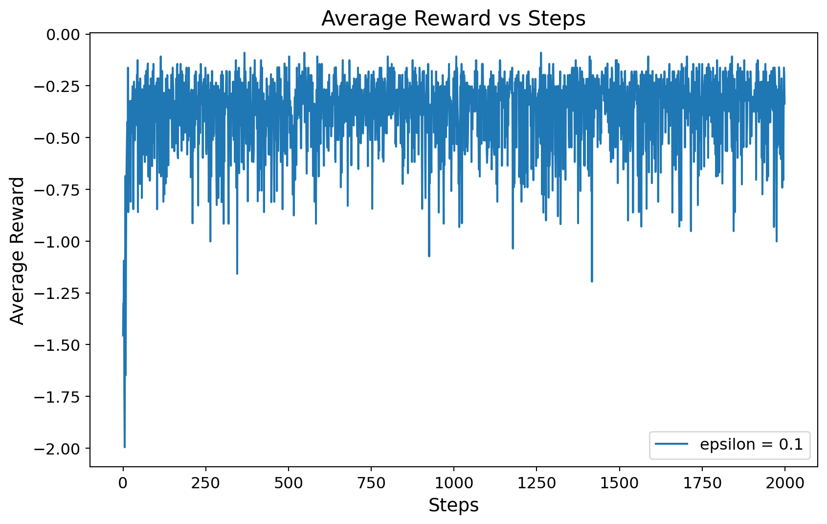
We set the planning horizon steps = 2000. We use the \epsilon-greedy policy with \epsilon = 0.1. We run the algorithm 10 times by setting number_of_runs = 10 and store the results in the rewards array. Finally, we plot the average reward over time.

import numpy as np
import matplotlib.pyplot as plt


class newsvendor_as_bandits:
    def __init__(self, k, h, p, mu, sigma):
        self.k = k
        self.h = h
        self.p = p
        self.mu = mu
        self.sigma = sigma

    def bandit(self, action):
        # sample demand to integer
        demand = round(np.random.normal(self.mu, self.sigma))
        # calculate cost
        cost = self.h * max(action - demand, 0) + self.p * max(demand - action, 0)
        return -cost


class bandit_algorithm:
    def __init__(self, bandit, epsilon, steps):
        self.bandit = bandit
        self.epsilon = epsilon
        self.steps = steps
        self.k = bandit.k
        self.Q = np.zeros(self.k)
        self.N = np.zeros(self.k)
        self.reward = np.zeros(self.steps)

    def learn(self):
        for t in range(self.steps):
            # epsilon greedy
            if np.random.rand() < self.epsilon:
                action = np.random.randint(self.k)
            else:
                # choose action with maximum Q, if multiple, choose randomly
                action = np.random.choice(np.where(self.Q == np.max(self.Q))[0])
            # get reward
            reward = self.bandit.bandit(action)
            # update Q
            self.N[action] += 1
            self.Q[action] += (reward - self.Q[action]) / self.N[action]
            # update reward
            self.reward[t] = reward


if __name__ == "__main__":

    # set random seed for reproducibility
    np.random.seed(0)

    # parameters
    k = 10
    h = 0.18
    p = 0.7
    mu = 5
    sigma = 1
    optimal = 6
    epsilon_list = [0.1]
    steps = 2000

    # mean reward
    number_of_runs = 10
    rewards = np.zeros((len(epsilon_list), number_of_runs, steps))

    # newsvendor problem
    newsvendor = newsvendor_as_bandits(k, h, p, mu, sigma)

    for i in range(len(epsilon_list)):
        for j in range(number_of_runs):
            # initialize bandit algorithm
            bandit = bandit_algorithm(newsvendor, epsilon_list[i], steps)
            # learn
            bandit.learn()
            # store results
            rewards[i, j, :] = bandit.reward
            # print optimal action and Q value
            print(
                "optimal action = {}, Q = {}".format(
                    np.argmax(bandit.Q), bandit.Q[np.argmax(bandit.Q)]
                )
            )

    # plot
    plt.figure(figsize=(10, 6))
    for i in range(len(epsilon_list)):
        plt.plot(
            np.mean(rewards[i, :, :], axis=0),
            label="epsilon = {}".format(epsilon_list[i]),
        )
    plt.xlabel("Steps", fontsize=14)
    plt.ylabel("Average Reward", fontsize=14)
    plt.title("Average Reward vs Steps", fontsize=16)
    plt.tick_params(axis="both", which="major", labelsize=12)
    plt.legend(fontsize=12)
    plt.show()

optimal action = 6, Q = -0.2510071942446042
optimal action = 6, Q = -0.2510820045558093
optimal action = 6, Q = -0.24312393887945655
optimal action = 6, Q = -0.24921290322580647
optimal action = 6, Q = -0.25454344216934205
optimal action = 6, Q = -0.24310325786858075
optimal action = 6, Q = -0.2506343077771653
optimal action = 6, Q = -0.24419944598337928
optimal action = 6, Q = -0.251546052631579
optimal action = 6, Q = -0.2518596881959912

References